Sentiment Analysis is one of the interesting applications of text analytics. Although the term is often associated with sentiment classification of documents, broadly speaking it refers to the use of text analytics approaches applied to the set of problems related to identifying and extracting subjective material in text sources.
This article continues the series on mining Twitter data with Python, describing a simple approach for Sentiment Analysis and applying it to the rubgy data set (see Part 4).
Tutorial Table of Contents:
- Part 1: Collecting data
- Part 2: Text Pre-processing
- Part 3: Term Frequencies
- Part 4: Rugby and Term Co-Occurrences
- Part 5: Data Visualisation Basics
- Part 6: Sentiment Analysis Basics (this article)
- Part 7: Geolocation and Interactive Maps
A Simple Approach for Sentiment Analysis
The technique we’re discussing in this post has been elaborated from the traditional approach proposed by Peter Turney in his paper Thumbs Up or Thumbs Down? Semantic Orientation Applied to Unsupervised Classification of Reviews. A lot of work has been done in Sentiment Analysis since then, but the approach has still an interesting educational value. In particular, it is intuitive, simple to understand and to test, and most of all unsupervised, so it doesn’t require any labelled data for training.
Firstly, we define the Semantic Orientation (SO) of a word as the difference between its associations with positive and negative words. In practice, we want to calculate “how close” a word is with terms like good and bad. The chosen measure of “closeness” is Pointwise Mutual Information (PMI), calculated as follows (t1 and t2 are terms):

In Turney’s paper, the SO of a word was calculated against excellent and poor, but of course we can extend the vocabulary of positive and negative terms. Using 


We can build our own list of positive and negative terms, or we can use one of the many resources available on-line, for example the opinion lexicon by Bing Liu.
Computing Term Probabilities
In order to compute 

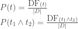
In the previous articles, the document frequency for single terms was stored in the dictionaries count_single and count_stop_single (the latter doesn’t store stop-words), while the document frequency for the co-occurrencies was stored in the co-occurrence matrix com
This is how we can compute the probabilities:
# n_docs is the total n. of tweets
p_t = {}
p_t_com = defaultdict(lambda : defaultdict(int))

for term, n in count_stop_single.items():
    p_t[term] = n / n_docs
    for t2 in com[term]:
        p_t_com[term][t2] = com[term][t2] / n_docs
Computing the Semantic Orientation
Given two vocabularies for positive and negative terms:
positive_vocab = [
    'good', 'nice', 'great', 'awesome', 'outstanding',
    'fantastic', 'terrific', ':)', ':-)', 'like', 'love',
    # shall we also include game-specific terms?
    # 'triumph', 'triumphal', 'triumphant', 'victory', etc.
]
negative_vocab = [
    'bad', 'terrible', 'crap', 'useless', 'hate', ':(', ':-(',
    # 'defeat', etc.
]
We can compute the PMI of each pair of terms, and then compute the
Semantic Orientation as described above:
pmi = defaultdict(lambda : defaultdict(int))
for t1 in p_t:
    for t2 in com[t1]:
        denom = p_t[t1] * p_t[t2]
        pmi[t1][t2] = math.log2(p_t_com[t1][t2] / denom)

semantic_orientation = {}
for term, n in p_t.items():
    positive_assoc = sum(pmi[term][tx] for tx in positive_vocab)
    negative_assoc = sum(pmi[term][tx] for tx in negative_vocab)
    semantic_orientation[term] = positive_assoc - negative_assoc
The Semantic Orientation of a term will have a positive (negative) value if the term is often associated with terms in the positive (negative) vocabulary. The value will be zero for neutral terms, e.g. the PMI’s for positive and negative balance out, or more likely a term is never observed together with other terms in the positive/negative vocabularies.
We can print out the semantic orientation for some terms:
semantic_sorted = sorted(semantic_orientation.items(),
                         key=operator.itemgetter(1),
                         reverse=True)
top_pos = semantic_sorted[:10]
top_neg = semantic_sorted[-10:]

print(top_pos)
print(top_neg)
print("ITA v WAL: %f" % semantic_orientation['#itavwal'])
print("SCO v IRE: %f" % semantic_orientation['#scovire'])
print("ENG v FRA: %f" % semantic_orientation['#engvfra'])
print("#ITA: %f" % semantic_orientation['#ita'])
print("#FRA: %f" % semantic_orientation['#fra'])
print("#SCO: %f" % semantic_orientation['#sco'])
print("#ENG: %f" % semantic_orientation['#eng'])
print("#WAL: %f" % semantic_orientation['#wal'])
print("#IRE: %f" % semantic_orientation['#ire'])
Different vocabularies will produce different scores. Using the opinion lexicon from Bing Liu, this is what we can observed on the Rugby data-set:
# the top positive terms
[('fantastic', 91.39950482011552), ('@dai_bach', 90.48767241244532), ('hoping', 80.50247748725415), ('#it', 71.28333427277785), ('days', 67.4394844955977), ('@nigelrefowens', 64.86112716005566), ('afternoon', 64.05064208341855), ('breathtaking', 62.86591435212975), ('#wal', 60.07283361352875), ('annual', 58.95378954406133)]
# the top negative terms
[('#england', -74.83306534609066), ('6', -76.0687215594536), ('#itavwal', -78.4558633116863), ('@rbs_6_nations', -80.89363516601993), ("can't", -81.75379628180468), ('like', -83.9319149443813), ('10', -85.93073078165587), ('italy', -86.94465165178258), ('#engvfra', -113.26188957010228), ('ball', -161.82146824640125)]
# Matches
ITA v WAL: -78.455863
SCO v IRE: -73.487661
ENG v FRA: -113.261890
# Individual team
#ITA: 53.033824
#FRA: 14.099372
#SCO: 4.426723
#ENG: -0.462845
#WAL: 60.072834
#IRE: 19.231722
Some Limitations
The PMI-based approach has been introduced as simple and intuitive, but of course it has some limitations. The semantic scores are calculated on terms, meaning that there is no notion of “entity” or “concept” or “event”. For example, it would be nice to aggregate and normalise all the references to the team names, e.g. #ita, Italy and Italia should all contribute to the semantic orientation of the same entity. Moreover, do the opinions on the individual teams also contribute to the overall opinion on a match?
Some aspects of natural language are also not captured by this approach, more notably modifiers and negation: how do we deal with phrases like not bad (this is the opposite of just bad) or very good (this is stronger than just good)?
Summary
This article has continued the tutorial on mining Twitter data with Python introducing a simple approach for Sentiment Analysis, based on the computation of a semantic orientation score which tells us whether a term is more closely related to a positive or negative vocabulary. The intuition behind this approach is fairly simple, and it can be implemented using Pointwise Mutual Information as a measure of association. The approach has of course some limitations, but it’s a good starting point to get familiar with Sentiment Analysis.
- Part 1: Collecting data
- Part 2: Text Pre-processing
- Part 3: Term Frequencies
- Part 4: Rugby and Term Co-Occurrences
- Part 5: Data Visualisation Basics
- Part 6: Sentiment Analysis Basics (this article)
- Part 7: Geolocation and Interactive Maps

The implementation of PMI is memory inefficient, i don’t recommend using this for larger datasets.
LikeLiked by 1 person
Yes, numpy arrays instead of python dictionaries are advisable for anything bigger than a toy dataset
LikeLike
Hey Marco,
thanks a lot for this nice introduction!!
I have streamed some data from twitter over a period of 2 Weeks.
I kind of adjusted your code a bit for my matter.
If I analyze the data now, my code clusters all the tweets into 1 day packages and gives me the PMI for a certain word for that day.
The goal is to have a normalized set of pmi´s over a period of 14 days to see the difference in opinion between each day. If I dont normalize the data, the difference depends actually on the amount of tweets i have.
Therefore i want to normalize the pmi, the line looks like that:
pmi[t1][t2] = (math.log2(p_t_com[t1][t2] / denom)/(-(math.log2(p_t_com[t1][t2]))))
is that formula correct?
Now the value of all co-occurences is between -1 and 1, correct?
If i add up all the different PMI´s of the co-occurence words which come together with that particular one i end up having a PMI still depending on the number of tweets i collect.
positive_assoc = sum(pmi[term][tx] for tx in positive_vocab)
negative_assoc = sum(pmi[term][tx] for tx in negative_vocab)
semantic_orientation[term] = (positive_assoc – negative_assoc)/count2
So i have to divide this PMI through the number of elements i added up?
Is that right? Or do you have another suggestion? I am just a little bit lost…
Hopefully you understand my problem, my english is not the best!
LikeLike
Hi Marco,
very nice articles.
Just a question here: is there a possibility to print a hole Tweet with positiv words
and not just the positiv / negative words alone?
LikeLike
Hi pad, yes you can loop through the tweets again after building the vocabularies (e.g. top_pos and top_neg in the last example), and it’s a matter of checking:
if any(word in tweet[‘text’] for word in top_pos):
print(tweet[‘text’])
LikeLike
hey marco, thank you i will try this.
when you’ re printing out your PMI’s do you get the same results everytime?
I once hat a PMI of -1.853720 and the next time 18.056733 for the same term :O
LikeLike
Assuming the data set is the same, and the vocabularies V+ and V- are the same, you should end up with the same values for PMI. With different data (e.g. new tweets added to the data set) the term probabilities are most likely to be different
LikeLike
hmm I’m using the same dataset and becoming different pmi’s every time
LikeLike
Thank you for a nice post. I really liked it.
LikeLike
Hello again!
As usual, I have another question.
The co-occurrence dict give the occurrence of two words that occur in the same tweet. I read the paper and it stated we use 2 words for somewhat deriving the context, and hence we look at 2 consecutive words. Doesn’t that mean we should use something like this in finding the co-occurances instead of using 2 for loops?
#editing com
for i in range(len(word_list)-1):
word1, word2 = sorted([ word_list[i], word_list[ i+1 ]])
if word1 != word2:
com[word1][word2] +=1
LikeLike
Hi Krishanu, the approach using a local context can be useful to extract phrases that follow a particular pattern (e.g. an adjective followed by a noun, for example “good movie”). If you follow this route, the downside is that you need to specify all these patterns manually. Experimenting with bigrams/trigrams is indeed worth exploring, but consider that you can fall short in many occasions. For example in the sentence “the movie was very good”, the connection movie-good is not captured by bigrams/trigrams because the two words are too distant. It makes sense to consider local context in reviews that can span multiple sentences, maybe less in a tweet that has just a few words. Long story short, try it :)
It’s worth mentioning that there are also more advanced techniques, like word2vec, used to better represent words and to capture semantic relationships between words — I just haven’t had much time to write about it.
Cheers,
Marco
LikeLike
Can somebody just reply with the hole conding until now because i can’t compile it thnx
LikeLike
does not work any help plzzzzzzzzzzzz
—————————————-
import sys
import json
from collections import Counter
import re
from nltk.corpus import stopwords
import string
from collections import defaultdict
import operator
p_t = {}
p_t_com = defaultdict(lambda : defaultdict(int))
com = defaultdict(lambda : defaultdict(int))
pmi = defaultdict(lambda : defaultdict(int))
punctuation = list(string.punctuation)
stop = stopwords.words(‘english’) + punctuation + [‘rt’, ‘via’]
emoticons_str = r”””
(?:
[:=;] # Eyes
[oO\-]? # Nose (optional)
[D\)\]\(\]/\\OpP] # Mouth
)”””
regex_str = [
emoticons_str,
r’]+>’, # HTML tags
r'(?:@[\w_]+)’, # @-mentions
r”(?:\#+[\w_]+[\w\’_\-]*[\w_]+)”, # hash-tags
r’http[s]?://(?:[a-z]|[0-9]|[$-_@.&+]|[!*\(\),]|(?:%[0-9a-f][0-9a-f]))+’, # URLs
r'(?:(?:\d+,?)+(?:\.?\d+)?)’, # numbers
r”(?:[a-z][a-z’\-_]+[a-z])”, # words with – and ‘
r'(?:[\w_]+)’, # other words
r'(?:\S)’ # anything else
]
tokens_re = re.compile(r'(‘+’|’.join(regex_str)+’)’, re.VERBOSE | re.IGNORECASE)
emoticon_re = re.compile(r’^’+emoticons_str+’$’, re.VERBOSE | re.IGNORECASE)
def tokenize(s):
return tokens_re.findall(s)
def preprocess(s, lowercase=True):
tokens = tokenize(s)
if lowercase:
tokens = [token if emoticon_re.search(token) else token.lower() for token in tokens]
return tokens
if __name__ == ‘__main__’:
fname = ‘news.json’
with open(fname, ‘r’) as f:
count_stop_single = Counter()
for line in f:
tweet = json.loads(line)
terms_only = [term for term in preprocess(tweet[‘text’])
if term not in stop and
not term.startswith((‘#’, ‘@’, ‘http’)) and
len(term) > 2]
# Build co-occurrence matrix
for i in range(len(terms_only)-1):
for j in range(i+1, len(terms_only)):
w1, w2 = sorted([terms_only[i], terms_only[j]])
if w1 != w2:
com[w1][w2] += 1
com_max = []
# For each term, look for the most common co-occurrent terms
for t1 in com:
t1_max_terms = sorted(com[t1].items(), key=operator.itemgetter(1), reverse=True)[:5]
for t2, t2_count in t1_max_terms:
com_max.append(((t1, t2), t2_count))
terms_max = sorted(com_max, key=operator.itemgetter(1), reverse=True)
print(terms_max[:5])
#
for term, n in count_stop_single.items():
p_t[term] = n / n_docs
for t2 in com[term]:
p_t_com[term][t2] = com[term][t2] / n_docs
print(p_t_com[term][t2]
positive_vocab = [
‘good’, ‘nice’, ‘great’, ‘awesome’, ‘outstanding’,
‘fantastic’, ‘terrific’, ‘:)’, ‘:-)’, ‘like’, ‘love’,
# shall we also include game-specific terms?
# ‘triumph’, ‘triumphal’, ‘triumphant’, ‘victory’, etc.
]
negative_vocab = [
‘bad’, ‘terrible’, ‘crap’, ‘useless’, ‘hate’, ‘:(‘, ‘:-(‘,
# ‘defeat’, etc.
]
for t1 in p_t:
for t2 in com[t1]:
denom = p_t[t1] * p_t[t2]
pmi[t1][t2] = math.log2(p_t_com[t1][t2] / denom)
semantic_orientation = {}
for term, n in p_t.items():
positive_assoc = sum(pmi[term][tx] for tx in positive_vocab)
negative_assoc = sum(pmi[term][tx] for tx in negative_vocab)
semantic_orientation[term] = positive_assoc – negative_assoc
semantic_sorted = sorted(semantic_orientation.items(),
key=operator.itemgetter(1),
reverse=True)
top_pos = semantic_sorted[:10]
top_neg = semantic_sorted[-10:]
print(top_pos)
print(top_neg)
print(“this: %f” % semantic_orientation[‘#new’])
print(“SCO v IRE: %f” % semantic_orientation[‘#scovire’])
print(“ENG v FRA: %f” % semantic_orientation[‘#engvfra’])
print(“#ITA: %f” % semantic_orientation[‘#ita’])
print(“#FRA: %f” % semantic_orientation[‘#fra’])
print(“#SCO: %f” % semantic_orientation[‘#sco’])
print(“#ENG: %f” % semantic_orientation[‘#eng’])
print(“#WAL: %f” % semantic_orientation[‘#wal’])
print(“#IRE: %f” % semantic_orientation[‘#ire’])
LikeLike
Did you ever got this to work?
LikeLike
Hi Kel3vra, do you have a specific error? Is your news.json file well formed?
LikeLike
my json is ok because is working with the other scripts from previous parts… the problem is can’t understand with which of yours previous scripts i must attach the semantic orientation to work correctly. I post my code which is basics yours from the article but i think is completely wrong the only change is the json file… i get this output
[]
[]
Traceback (most recent call last):
File “C:\Python27\Datamine\SemOr.py”, line 112, in
print(“ITA v WAL: %f” % semantic_orientation[‘#itavwal’])
KeyError: ‘#itavwal’
LikeLike
This is incredible… Thank you!
LikeLike
Hi, I’m using Python 2.7 and it doesn’t allow log2:
“pmi[t1][t2] = math.log2(p_t_com[t1][t2] / denom)”
So I’m using “pmi[t1][t2] = math.log(p_t_com[t1][t2] / denom) / math.log(2)” instead… but I receive this error…
pmi[t1][t2] = math.log(p_t_com[t1][t2] / denom) / math.log(2)
ZeroDivisionError: integer division or modulo by zero
any idea how to get around this?
Thanks… I’ve been learning immensely from this blog. Most of this stuff is way over my head but I find it so interesting.
LikeLike
Managed to solve it by “from __future__ import division” :-)
Thanks again Marco… you are my favorite genius!!!
LikeLike
Hi Mandla, glad you solved it. Thanks for the nice words
Cheers,
Marco
LikeLike
Hey Marco, Mandla again…
I would like to know what the measuring unit is for Semantic Orientation and/or how can it be represented as a percentage?
LikeLike
Hi Mandla, the SO has no particular measuring unit. It’s defined through the Pointwise Mutual Information (PMI) formula as described above and in the paper by P.Turney linked in the article. If you check out the wikipedia page for PMI (https://en.wikipedia.org/wiki/Pointwise_mutual_information), there are option to normalise it, which I haven’t used. In summary, SO is a simple way to give you a hint about the polarity of words.
Cheers,
Marco
LikeLike
Hi! Amazing tutorial!
I did not understand this snipped though –
# n_docs is the total n. of tweets
p_t = {}
p_t_com = defaultdict(lambda : defaultdict(int))
for term, n in count_stop_single.items():
p_t[term] = n / n_docs
for t2 in com[term]:
p_t_com[term][t2] = com[term][t2] / n_docs
What is n_docs here?
Thanks!!
LikeLike
Hi Nachiket
n_docs is the total number of tweets that you have collected. If you’re streaming into a JSON Lines file as described in the previous articles, it’s essentially the total number of lines in that file.
Cheers
Marco
LikeLike
I want to generate 2 million tweet using r,please can u help me out. thanks in anticipation
LikeLike
where is count_stop_single dictionary i cant find it!
LikeLike