Mining Twitter Data with Python (Part 6 – Sentiment Analysis Basics)

Sentiment Analysis is one of the interesting applications of text analytics. Although the term is often associated with sentiment classification of documents, broadly speaking it refers to the use of text analytics approaches applied to the set of problems related to identifying and extracting subjective material in text sources.

This article continues the series on mining Twitter data with Python, describing a simple approach for Sentiment Analysis and applying it to the rubgy data set (see Part 4).

Tutorial Table of Contents:

A Simple Approach for Sentiment Analysis

The technique we’re discussing in this post has been elaborated from the traditional approach proposed by Peter Turney in his paper Thumbs Up or Thumbs Down? Semantic Orientation Applied to Unsupervised Classification of Reviews. A lot of work has been done in Sentiment Analysis since then, but the approach has still an interesting educational value. In particular, it is intuitive, simple to understand and to test, and most of all unsupervised, so it doesn’t require any labelled data for training.

Firstly, we define the Semantic Orientation (SO) of a word as the difference between its associations with positive and negative words. In practice, we want to calculate “how close” a word is with terms like good and bad. The chosen measure of “closeness” is Pointwise Mutual Information (PMI), calculated as follows (t1 and t2 are terms):

\mbox{PMI}(t_1, t_2) = \log\Bigl(\frac{P(t_1 \wedge t_2)}{P(t_1) \cdot P(t_2)}\Bigr)

In Turney’s paper, the SO of a word was calculated against excellent and poor, but of course we can extend the vocabulary of positive and negative terms. Using V^{+} and a vocabulary of positive terms and V^{-} for the negative ones, the Semantic Orientation of a term t is hence defined as:

\mbox{SO}(t) = \sum_{t' \in V^{+}}\mbox{PMI}(t, t') - \sum_{t' \in V^{-}}\mbox{PMI}(t, t')

We can build our own list of positive and negative terms, or we can use one of the many resources available on-line, for example the opinion lexicon by Bing Liu.

Computing Term Probabilities

In order to compute P(t) (the probability of observing the term t) and P(t_1 \wedge t_2) (the probability of observing the terms t1 and t2 occurring together) we can re-use some previous code to calculate term frequencies and term co-occurrences. Given the set of documents (tweets) D, we define the Document Frequency (DF) of a term as the number of documents where the term occurs. The same definition can be applied to co-occurrent terms. Hence, we can define our probabilities as:

P(t) = \frac{\mbox{DF}(t)}{|D|}\\  P(t_1 \wedge t_2) = \frac{\mbox{DF}(t_1 \wedge t_2)}{|D|}

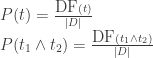
In the previous articles, the document frequency for single terms was stored in the dictionaries count_single and count_stop_single (the latter doesn’t store stop-words), while the document frequency for the co-occurrencies was stored in the co-occurrence matrix com

This is how we can compute the probabilities:

# n_docs is the total n. of tweets
p_t = {}
p_t_com = defaultdict(lambda : defaultdict(int))

for term, n in count_stop_single.items():
    p_t[term] = n / n_docs
    for t2 in com[term]:
        p_t_com[term][t2] = com[term][t2] / n_docs

Computing the Semantic Orientation

Given two vocabularies for positive and negative terms:

positive_vocab = [
    'good', 'nice', 'great', 'awesome', 'outstanding',
    'fantastic', 'terrific', ':)', ':-)', 'like', 'love',
    # shall we also include game-specific terms?
    # 'triumph', 'triumphal', 'triumphant', 'victory', etc.
]
negative_vocab = [
    'bad', 'terrible', 'crap', 'useless', 'hate', ':(', ':-(',
    # 'defeat', etc.
]

We can compute the PMI of each pair of terms, and then compute the
Semantic Orientation as described above:

pmi = defaultdict(lambda : defaultdict(int))
for t1 in p_t:
    for t2 in com[t1]:
        denom = p_t[t1] * p_t[t2]
        pmi[t1][t2] = math.log2(p_t_com[t1][t2] / denom)

semantic_orientation = {}
for term, n in p_t.items():
    positive_assoc = sum(pmi[term][tx] for tx in positive_vocab)
    negative_assoc = sum(pmi[term][tx] for tx in negative_vocab)
    semantic_orientation[term] = positive_assoc - negative_assoc

The Semantic Orientation of a term will have a positive (negative) value if the term is often associated with terms in the positive (negative) vocabulary. The value will be zero for neutral terms, e.g. the PMI’s for positive and negative balance out, or more likely a term is never observed together with other terms in the positive/negative vocabularies.

We can print out the semantic orientation for some terms:

semantic_sorted = sorted(semantic_orientation.items(), 
                         key=operator.itemgetter(1), 
                         reverse=True)
top_pos = semantic_sorted[:10]
top_neg = semantic_sorted[-10:]

print(top_pos)
print(top_neg)
print("ITA v WAL: %f" % semantic_orientation['#itavwal'])
print("SCO v IRE: %f" % semantic_orientation['#scovire'])
print("ENG v FRA: %f" % semantic_orientation['#engvfra'])
print("#ITA: %f" % semantic_orientation['#ita'])
print("#FRA: %f" % semantic_orientation['#fra'])
print("#SCO: %f" % semantic_orientation['#sco'])
print("#ENG: %f" % semantic_orientation['#eng'])
print("#WAL: %f" % semantic_orientation['#wal'])
print("#IRE: %f" % semantic_orientation['#ire'])

Different vocabularies will produce different scores. Using the opinion lexicon from Bing Liu, this is what we can observed on the Rugby data-set:

# the top positive terms
[('fantastic', 91.39950482011552), ('@dai_bach', 90.48767241244532), ('hoping', 80.50247748725415), ('#it', 71.28333427277785), ('days', 67.4394844955977), ('@nigelrefowens', 64.86112716005566), ('afternoon', 64.05064208341855), ('breathtaking', 62.86591435212975), ('#wal', 60.07283361352875), ('annual', 58.95378954406133)]
# the top negative terms
[('#england', -74.83306534609066), ('6', -76.0687215594536), ('#itavwal', -78.4558633116863), ('@rbs_6_nations', -80.89363516601993), ("can't", -81.75379628180468), ('like', -83.9319149443813), ('10', -85.93073078165587), ('italy', -86.94465165178258), ('#engvfra', -113.26188957010228), ('ball', -161.82146824640125)]
# Matches
ITA v WAL: -78.455863
SCO v IRE: -73.487661
ENG v FRA: -113.261890
# Individual team
#ITA: 53.033824
#FRA: 14.099372
#SCO: 4.426723
#ENG: -0.462845
#WAL: 60.072834
#IRE: 19.231722

Some Limitations

The PMI-based approach has been introduced as simple and intuitive, but of course it has some limitations. The semantic scores are calculated on terms, meaning that there is no notion of “entity” or “concept” or “event”. For example, it would be nice to aggregate and normalise all the references to the team names, e.g. #ita, Italy and Italia should all contribute to the semantic orientation of the same entity. Moreover, do the opinions on the individual teams also contribute to the overall opinion on a match?

Some aspects of natural language are also not captured by this approach, more notably modifiers and negation: how do we deal with phrases like not bad (this is the opposite of just bad) or very good (this is stronger than just good)?

Summary

This article has continued the tutorial on mining Twitter data with Python introducing a simple approach for Sentiment Analysis, based on the computation of a semantic orientation score which tells us whether a term is more closely related to a positive or negative vocabulary. The intuition behind this approach is fairly simple, and it can be implemented using Pointwise Mutual Information as a measure of association. The approach has of course some limitations, but it’s a good starting point to get familiar with Sentiment Analysis.

@MarcoBonzanini

Sentiment Analysis with Python and scikit-learn

Sentiment Analysis is a field of study which analyses people’s opinions towards entities like products, typically expressed in written forms like on-line reviews. In recent years, it’s been a hot topic in both academia and industry, also thanks to the massive popularity of social media which provide a constant source of textual data full of opinions to analyse.

This article discusses one particular application of sentiment analysis: sentiment classification at the document level. In other words, given a document (e.g. a review), the task consists in finding out whether it provides a positive or a negative sentiment towards the product being discussed.

The following paragraphs describe the setup and the main components
or our classification example with samples of code in Python using scikit-learn, a popular machine learning library. The complete code is discussed at the end of this post, and available as Gist on Github.

Setting up for the experiments

We’re using Python and in particular scikit-learn for these experiments. To install scikit-learn:

pip install -U scikit-learn

Scikit-learn has a couple of dependencies, in particular numpy and scipy. If these dependencies are not resolved by pip for some reason, you can make the installation explicit with:

pip install -U numpy scipy scikit-learn

The data set used for this experiments is the well-known Polarity Dataset v2.0, downloadable from here.

The data set contains 2,000 documents, labelled and pre-processed. In particular, there are two labels, positive and negative with 1,000 documents each. Every document has been tokenised and lowercased; each line of a document represents a sentence. This pre-processing takes out most of the work we have to do to get started, so we can focus on the classification problem. Real world data are usually messy and need proper pre-processing before we can make good use of them. All we need to do here is read the files and split the words over white spaces.

Feature extraction in scikit-learn

In classification, items are represented by their features. In our case, documents are represented by their words, so we will use words as features.

scikit-learn provides several vectorizers to translate the input documents into vectors of features (or feature weights). Typically we want to give appropriate weights to different words, and TF-IDF is one of the most common weighting schemes used in text analytics applications. In scikit-learn, we can use the TfidfVectorizer:

vectorizer = TfidfVectorizer(min_df=5,
                             max_df = 0.8,
                             sublinear_tf=True,
                             use_idf=True)
train_vectors = vectorizer.fit_transform(train_data)
test_vectors = vectorizer.transform(test_data)

The parameters used in this example with the vectorizer are:

  • min_df=5, discard words appearing in less than 5 documents
  • max_df=0.8, discard words appering in more than 80% of the documents
  • sublinear_tf=True, use sublinear weighting
  • use_idf=True, enable IDF

More options are available and the best configuration might depend on your data or on the details of the task you’re facing.

The first call to fit_transform() will create the vocabulary (i.e. the list of words/features) and the feature weights from the training data. Secondly, we call simply transform() on the test data, which will create the feature weights for the test data, using the same vocabulary as the training data.

Classification in scikit-learn

scikit-learn comes with a number of different classifiers already built-in. In these experiments, we use different variations of Support Vector Machine (SVM), which is commonly used in classification applications.

The classification procedure is fairly simple:

classifier_rbf = svm.SVC()
classifier_rbf.fit(train_vectors, train_labels)
prediction_rbf = classifier_rbf.predict(test_vectors)

The SVC() class generates a SVM classifier with RBF (Gaussian) kernel as default option (several other options are available).

The fit() method will perform the training and it requires the training data processed by the vectorizer as well as the correct class labels.

The classification step consists in predicting the labels for the test data.

Comments on The Complete Code

The complete code is available as Gist on Github. The script takes the data folder as parameter, assuming the same format of the original data, with two subfolders pos and neg.

The first reads the content of the files and creates lists of training/testing documents and labels.
We split the data set into training (90% of the documents) and testing (10%) by exploiting the file names (they all start with “cvX”, with X=[0..9]). This calls for k-fold cross-validation,
not implemented in the example but fairly easy to integrate.

if fname.startswith('cv9'):
    # 10% test data
    test_data.append(content)
    test_labels.append(curr_class)
else:
    # 90% training data
    train_data.append(content)
    train_labels.append(curr_class)

Once the vectorizer has generated the feature vectors for training and testing, we can call the classifier as described above. In the example, we try different variations of SVM:

classifier_rbf = svm.SVC()
classifier_linear = svm.SVC(kernel='linear')
classifier_liblinear = svm.LinearSVC()

After performing the classification, we print the quality (precision/recall) results using classification_report(), and some timing information.

We notice that:

  • The default RBG kernel performs worse than the linear kernel
  • SVC() with linear kernel is much much slower than LinearSVC()

The first point opens for a discussion on Gaussian vs. linear kernels, not really part of this blog post, but as a rule of thumb when the number of features is much higher than the number of samples (documents), a linear kernel is probably the preferred choice. Moreover, there are options to properly tune the parameters of a RBF kernel.

The second bullet point is easily explained by the fact that, under the hood, scikit-learn relies on different C libraries. In particular SVC() is implemented using libSVM, while LinearSVC() is implemented using liblinear, which is explicitly designed for this kind of application.

Summary

We have discussed an application of sentiment analysis, tackled as a document classification problem with Python and scikit-learn.

The choice of the classifier, as well as the feature extraction process, will influence the overall quality of the results, and it’s always good to experiment with different configurations.

scikit-learn offers many options from this point of view.

Knowing the underlying implementation also allows for a better choice in terms of speed.

Full example in Python.