PyCon Italy 2017 write-up

Last week I’ve travelled to Florence where I attended PyCon Otto, the 8th edition of the Italian Python Conference. As expected, it’s been yet another great experience with the Italian Python community and many international guests.

This year the very first day, Thursday, was beginners’ day, with introductory workshops run by volunteer mentors. Thanks to a cancelled flight, I’ve missed out on this opportunity so I joined the party only for the main event.

On Friday, I’ve run another version of my tutorial on Natural Language Processing for beginners. The tutorial was oversubscribed and the organisers really made an effort to accommodate as many people as possible in the small training room, so at the end, I had ~35 attendees. After the workshop, I had a lot of interesting conversations and some ideas on how to improve the material with additional exercises. Some credits for this are due to my friend Miguel Martinez who contributed with the text classification material for the first edition of the workshop.

As per tradition, at the end of the workshop I’ve also run a raffle to give away a free copy of my book on Mastering Social Media Mining with Python.

On Saturday, I gave a talk titled Word Embeddings for Natural Language Processing with Python (link to slides), somehow a natural follow-up of the tutorial with slightly more advanced concepts, but still tailored for beginners. The talk was really well received, and a lot of interesting questions and conversations came up.

Following the traditional social event on Saturday night (a huge fiorentina), Sunday was pretty much a mellow day, with the last few excellent talks, a light lunch and my journey back.

It was great to meet so many new and old friends! The quality of this community event was stellar, and this was possible thanks to the contributions of organisers, volunteers, mentors, speakers and all the attendees.

See you for PyCon Italy 2018!

PyCon UK 2016 write-up

Last week I had a long weekend at PyCon UK 2016 in Cardiff, and it’s been a fantastic experience! Great talks, great friends/colleagues and lots of ideas.

On Monday 19th, on the last day of the conference, my friend Miguel and I have run a tutorial/workshop on Natural Language Processing in Python (the GitHub repo contains the Jupyter notebooks we used as well as some slides for an introduction).

Our NLP tutorial

Since I’ve already mentioned it, I’ll start from the end :)

The tutorial was tailored for NLP beginners and, as I mentioned explicitly at the very beginning, I wasn’t there to impress the experts. Rather, the whole point was to get the attendees a bit curious about Natural Language Processing, and to show them what you can do with a few lines of Python.

Overall, I think we’ve been quite lucky as we had the perfect audience: the right number of people (around 20+) with a bit of Python knowledge but not much NLP knowledge.

We only had some minor hiccups with the installation process, which is something we’re going to work on to make it smoother and more beginner-friendly. In particular the things I’d like to improve are:

  • add some testing / pre-flight checks, e.g. “how do I know that the environment is set up correctly?” (Miguel has already added this)
  • support for Windows: I’m quite useless with trouble-shooting Windows issues, but a couple of attendees had some troubles with the installation process not going too smoothly; maybe some virtual machine setup will be helpful

I also think having the material available in advance, so the attendees can start setting up the environment is very helpful. Most of them were quite engaged and I received a couple of “bug reports” on-the-fly, even a pull request that improved the installation process (thanks!)

Last but not least, I was also happy to give out a copy of my book (Mastering Social Media Mining with Python) that I had with me (the raffle was implemented on the spot through random.choice(), and the book went to Paivi from Django Girls).

I’ll give a shorter version of this tutorial at PyCon Ireland later this year, so in case you’ll be around, I’ll see you there :)

Unfortunately, the tutorials were not recorded so there is no video on-line, but the slides are in the GitHub repo so please dig in and send feedback if you have any.

The Open Day

Thursday 15th was “day zero” of the conference, hosted at Cardiff University. The ticket was free, although there was limited capacity. The day was aimed at introducing the new audience to Python and PyCon. We haven’t seen much Python code on that day, as the talks were mainly for newcomers, yet we had a lot of food for thoughs. This is a great way to introduce more people to Python and to show them how the community is friendly and happy to get more beginners on board.

Teachers, Kids and Education

One of the main themes of the conference was Education. Friday 16th, the first day of the main event, was labelled “Teachers Day”, while Saturday 17th was “Kids Day”. The effort to make CS education more accessible for kids was very clear, and some of the initiatives were really spot-on. In particular, some of the kids have been able to hack some small project together in a very short time, and they delivered a “show and tell” session at the end of the second day. I think their creativity and the fact that they were standing in front of a crowd of 500+ developers to show what they have been working on during their day have been very impressive.

Community in the Broader Sense

Another aspect that became quite clear is the strength of the Python Community. Some representatives of PyCon Poland, PyCon Switzerland and Django Europe were introducing their upcoming events. Some attendees with less economic capabilities were given the opportunity to attend, through some form of financial support (including e.g. students from India).

Representatives from PyCon Namibia and PyCon Zimbabwe were also attending and they discussed some of the challenges they are facing while building a local community in their countries.

In particular, the work Jessica from PyNAM is carrying out with young learners is extremely inspiring and deserves more visibility (link to the video of her talk).

Accessibility for Everybody

One of the features that I’ve never experienced in a conference so far was the speech-to-text transcription. During the talks, the speech-to-text team have been very busy writing down what the speakers were saying in real-time. While this is sometimes considered an accessibility feature which might benefit only deaf users, it turned out live captions are extremely beneficial for everybody. Firstly, not all the non-deaf attendees have perfect hearing. Secondly, not everybody is an English native speaker (both speakers and audience), so a word might be missed, or an accent might cause some confusion. Lastly, not every attendee is paying full attention to every talk for the whole talk: sometimes towards the end of the day, you just switch off for a moment and the live captions allow you to catch up.

Providing some accessibility feature turned out to be beneficial for everybody.

Shout out to the Organisers

Organising such a big event (500+ attendees) is not an easy task, so all the people who have worked hard to make this conference happen deserve a big round of applause. Not naming names here, but if you’ve been involved, thanks!

Being Interviewed about NLP

This was a bit random, in a very pleasant way. On Saturday, Miguel, Lev from RaRe Technologies and I spent some time with Kate Jarmul, who by the way just introduced her book on data wrangling, and also delivered a tutorial on the topic. The topic of the conversation was on our views, in the broader sense, about NLP / Text Analytics, how we got into this field, how we see this field evolving and so on. Apparently, this was an interview with some experts of the field, for a piece she’s writing for the O’Reilly blog (I should put an amazed emoticon here).

Using Python for …

The breadth of the topics discussed during the conference was really amazing. I think this kind of events are a great way to see what people are working on and how the tools we use every day are used by other people.

I’m not going to name any talk in particular, because there are too many good talks that deserve to be mentioned.

In terms of topics, some fields that are well covered by Python are:

  • Data Science (and related topics like data cleaning, NLP and machine learning)
  • Web development (with Django and so many interesting libraries)
  • electronics and robotics (with Raspberry Pi, micro:bit, MicroPython etc)
  • you name it :)

I’m probably not saying anything new here, but it was nice to see it in first person and step outside my data-sciency comfort zone.

Summary

Thanks to everybody who contributed to this event, and see you in Cardiff for PyCon UK 2017!

Mining Twitter Data with Python (Part 6 – Sentiment Analysis Basics)

Sentiment Analysis is one of the interesting applications of text analytics. Although the term is often associated with sentiment classification of documents, broadly speaking it refers to the use of text analytics approaches applied to the set of problems related to identifying and extracting subjective material in text sources.

This article continues the series on mining Twitter data with Python, describing a simple approach for Sentiment Analysis and applying it to the rubgy data set (see Part 4).

Tutorial Table of Contents:

A Simple Approach for Sentiment Analysis

The technique we’re discussing in this post has been elaborated from the traditional approach proposed by Peter Turney in his paper Thumbs Up or Thumbs Down? Semantic Orientation Applied to Unsupervised Classification of Reviews. A lot of work has been done in Sentiment Analysis since then, but the approach has still an interesting educational value. In particular, it is intuitive, simple to understand and to test, and most of all unsupervised, so it doesn’t require any labelled data for training.

Firstly, we define the Semantic Orientation (SO) of a word as the difference between its associations with positive and negative words. In practice, we want to calculate “how close” a word is with terms like good and bad. The chosen measure of “closeness” is Pointwise Mutual Information (PMI), calculated as follows (t1 and t2 are terms):

\mbox{PMI}(t_1, t_2) = \log\Bigl(\frac{P(t_1 \wedge t_2)}{P(t_1) \cdot P(t_2)}\Bigr)

In Turney’s paper, the SO of a word was calculated against excellent and poor, but of course we can extend the vocabulary of positive and negative terms. Using V^{+} and a vocabulary of positive terms and V^{-} for the negative ones, the Semantic Orientation of a term t is hence defined as:

\mbox{SO}(t) = \sum_{t' \in V^{+}}\mbox{PMI}(t, t') - \sum_{t' \in V^{-}}\mbox{PMI}(t, t')

We can build our own list of positive and negative terms, or we can use one of the many resources available on-line, for example the opinion lexicon by Bing Liu.

Computing Term Probabilities

In order to compute P(t) 
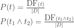
(the probability of observing the term t) and P(t_1 \wedge t_2) (the probability of observing the terms t1 and t2 occurring together) we can re-use some previous code to calculate term frequencies and term co-occurrences. Given the set of documents (tweets) D, we define the Document Frequency (DF) of a term as the number of documents where the term occurs. The same definition can be applied to co-occurrent terms. Hence, we can define our probabilities as:

P(t) = \frac{\mbox{DF}(t)}{|D|}\\  P(t_1 \wedge t_2) = \frac{\mbox{DF}(t_1 \wedge t_2)}{|D|}

In the previous articles, the document frequency for single terms was stored in the dictionaries count_single and count_stop_single (the latter doesn’t store stop-words), while the document frequency for the co-occurrencies was stored in the co-occurrence matrix com

This is how we can compute the probabilities:

# n_docs is the total n. of tweets
p_t = {}
p_t_com = defaultdict(lambda : defaultdict(int))

for term, n in count_stop_single.items():
    p_t[term] = n / n_docs
    for t2 in com[term]:
        p_t_com[term][t2] = com[term][t2] / n_docs

Computing the Semantic Orientation

Given two vocabularies for positive and negative terms:

positive_vocab = [
    'good', 'nice', 'great', 'awesome', 'outstanding',
    'fantastic', 'terrific', ':)', ':-)', 'like', 'love',
    # shall we also include game-specific terms?
    # 'triumph', 'triumphal', 'triumphant', 'victory', etc.
]
negative_vocab = [
    'bad', 'terrible', 'crap', 'useless', 'hate', ':(', ':-(',
    # 'defeat', etc.
]

We can compute the PMI of each pair of terms, and then compute the
Semantic Orientation as described above:

pmi = defaultdict(lambda : defaultdict(int))
for t1 in p_t:
    for t2 in com[t1]:
        denom = p_t[t1] * p_t[t2]
        pmi[t1][t2] = math.log2(p_t_com[t1][t2] / denom)

semantic_orientation = {}
for term, n in p_t.items():
    positive_assoc = sum(pmi[term][tx] for tx in positive_vocab)
    negative_assoc = sum(pmi[term][tx] for tx in negative_vocab)
    semantic_orientation[term] = positive_assoc - negative_assoc

The Semantic Orientation of a term will have a positive (negative) value if the term is often associated with terms in the positive (negative) vocabulary. The value will be zero for neutral terms, e.g. the PMI’s for positive and negative balance out, or more likely a term is never observed together with other terms in the positive/negative vocabularies.

We can print out the semantic orientation for some terms:

semantic_sorted = sorted(semantic_orientation.items(), 
                         key=operator.itemgetter(1), 
                         reverse=True)
top_pos = semantic_sorted[:10]
top_neg = semantic_sorted[-10:]

print(top_pos)
print(top_neg)
print("ITA v WAL: %f" % semantic_orientation['#itavwal'])
print("SCO v IRE: %f" % semantic_orientation['#scovire'])
print("ENG v FRA: %f" % semantic_orientation['#engvfra'])
print("#ITA: %f" % semantic_orientation['#ita'])
print("#FRA: %f" % semantic_orientation['#fra'])
print("#SCO: %f" % semantic_orientation['#sco'])
print("#ENG: %f" % semantic_orientation['#eng'])
print("#WAL: %f" % semantic_orientation['#wal'])
print("#IRE: %f" % semantic_orientation['#ire'])

Different vocabularies will produce different scores. Using the opinion lexicon from Bing Liu, this is what we can observed on the Rugby data-set:

# the top positive terms
[('fantastic', 91.39950482011552), ('@dai_bach', 90.48767241244532), ('hoping', 80.50247748725415), ('#it', 71.28333427277785), ('days', 67.4394844955977), ('@nigelrefowens', 64.86112716005566), ('afternoon', 64.05064208341855), ('breathtaking', 62.86591435212975), ('#wal', 60.07283361352875), ('annual', 58.95378954406133)]
# the top negative terms
[('#england', -74.83306534609066), ('6', -76.0687215594536), ('#itavwal', -78.4558633116863), ('@rbs_6_nations', -80.89363516601993), ("can't", -81.75379628180468), ('like', -83.9319149443813), ('10', -85.93073078165587), ('italy', -86.94465165178258), ('#engvfra', -113.26188957010228), ('ball', -161.82146824640125)]
# Matches
ITA v WAL: -78.455863
SCO v IRE: -73.487661
ENG v FRA: -113.261890
# Individual team
#ITA: 53.033824
#FRA: 14.099372
#SCO: 4.426723
#ENG: -0.462845
#WAL: 60.072834
#IRE: 19.231722

Some Limitations

The PMI-based approach has been introduced as simple and intuitive, but of course it has some limitations. The semantic scores are calculated on terms, meaning that there is no notion of “entity” or “concept” or “event”. For example, it would be nice to aggregate and normalise all the references to the team names, e.g. #ita, Italy and Italia should all contribute to the semantic orientation of the same entity. Moreover, do the opinions on the individual teams also contribute to the overall opinion on a match?

Some aspects of natural language are also not captured by this approach, more notably modifiers and negation: how do we deal with phrases like not bad (this is the opposite of just bad) or very good (this is stronger than just good)?

Summary

This article has continued the tutorial on mining Twitter data with Python introducing a simple approach for Sentiment Analysis, based on the computation of a semantic orientation score which tells us whether a term is more closely related to a positive or negative vocabulary. The intuition behind this approach is fairly simple, and it can be implemented using Pointwise Mutual Information as a measure of association. The approach has of course some limitations, but it’s a good starting point to get familiar with Sentiment Analysis.

@MarcoBonzanini

Some Thoughts on IWCS 2015

Last week I attended the 11th International Conference on Computational Semantics (IWCS 2015). This conference is the bi-yearly meeting of the ACL‘s Special Interest Group on Semantics and this edition was hosted by Queen Mary University’s Computational Linguistics Lab. The topics discussed at the conference revolve around computing, annotating, extracting and representing meaning in natural language. The format of the conference consisted in a first day of workshops (I attended Advances in Distributional Semantics, ADS) followed by three days of main event.

It was nice to be back at Queen Mary, where I studied for my MSc and PhD in Information Retrieval, and it was nice to have the opportunity to mix with a different academic crowd. In fact, a part from the local organisers, I hadn’t met any of the attendees before, and I only knew a couple of famous names. In particular, Hinrich Schuetze (probably best known for co-authoring a book on Natural Language Processing and one on Information Retrieval) gave a talk at the ADS workshop about The case against compositionality, and Yoshua Bengio (one of the most influencial figures in Deep Learning) gave one of the keynote speeches, about Deep Learning of Semantic Representations.

To confirm a feeling that I already had, I have to say that small, single-track conferences are in general more enjoyable than huge ones. You might not have an open bar reception in a 5+ stars fancy hotel, but the networking is much more relaxed, people are in general more approachable, and QA sessions are usually spot on. Of course it really depends on the venues, but my non-statistically significant experience tells me so. Moreover, in bigger venues a lot of attention goes to improving some baseline of some 0.1% accuracy (or whatever metric) without many details on the theoretical foundations (of course with exceptions). Smaller venues usually have the chance to dig deeper into what it is that really makes a model interesting, even when the results are less solid or the evaluation is on a small-ish scale.

Talking about evaluation, this was in my eyes the biggest difference with Information Retrieval conferences: scalability and large-scale evaluation have been rarely, if ever, mentioned. I understand that other venues like EMNLP are probably more suitable for these topics, but it was something that I noticed.

In general, it’s difficult to mention one particular talk, as they were all more or less interesting in my eyes, but one quote that stood out for me was an answer given by Prof. Bengio at the end of his keynote, regarding negation and quantification, and how a Neural Network model deals with them: “I don’t know. But it learns to do what it needs to do.”

As a final side-note, the social event/dinner was a boat trip on the Thames: looking at some well-known London landmarks from a different point of view was absolutely amazing. Well done to the organisers!

Mining Twitter Data with Python: Part 5 – Data Visualisation Basics

A picture is worth a thousand tweets: more often than not, designing a good visual representation of our data, can help us make sense of them and highlight interesting insights. After collecting and analysing Twitter data, the tutorial continues with some notions on data visualisation with Python.

Tutorial Table of Contents:

From Python to Javascript with Vincent

While there are some options to create plots in Python using libraries like matplotlib or ggplot, one of the coolest libraries for data visualisation is probably D3.js which is, as the name suggests, based on Javascript. D3 plays well with web standards like CSS and SVG, and allows to create some wonderful interactive visualisations.

Vincent bridges the gap between a Python back-end and a front-end that supports D3.js visualisation, allowing us to benefit from both sides. The tagline of Vincent is in fact “The data capabilities of Python. The visualization capabilities of JavaScript”. Vincent, a Python library, takes our data in Python format and translates them into Vega, a JSON-based visualisation grammar that will be used on top of D3. It sounds quite complicated, but it’s fairly simple and pythonic. You don’t have to write a line in Javascript/D3 if you don’t want to.

Firstly, let’s install Vincent:

pip install vincent

Secondly, let’s create our first plot. Using the list of most frequent terms (without hashtags) from our rugby data set, we want to plot their frequencies:

import vincent

word_freq = count_terms_only.most_common(20)
labels, freq = zip(*word_freq)
data = {'data': freq, 'x': labels}
bar = vincent.Bar(data, iter_idx='x')
bar.to_json('term_freq.json')

At this point, the file term_freq.json will contain a description of the plot that can be handed over to D3.js and Vega. A simple template (taken from Vincent resources) to visualise the plot:

<html>
<head>
    <title>Vega Scaffold</title>
    <script src="http://d3js.org/d3.v3.min.js" charset="utf-8"></script>
    <script src="http://d3js.org/topojson.v1.min.js"></script>
    <script src="http://d3js.org/d3.geo.projection.v0.min.js" charset="utf-8"></script>
    <script src="http://trifacta.github.com/vega/vega.js"></script>
</head>
<body>
    <div id="vis"></div>
</body>
<script type="text/javascript">
// parse a spec and create a visualization view
function parse(spec) {
  vg.parse.spec(spec, function(chart) { chart({el:"#vis"}).update(); });
}
parse("term_freq.json");
</script>
</html>

Save the above HTML page as chart.html and run the simple Python web server:

python -m http.server 8888 # Python 3
python -m SimpleHTTPServer 8888 # Python 2

Now you can open your browser at http://localhost:8888/chart.html and observe the result:

Term Frequencies

Notice: you could save the HTML template directly from Python with:

bar.to_json('term_freq.json', html_out=True, html_path='chart.html')

but, at least in Python 3, the output is not a well formed HTML and you’d need to manually strip some characters.

With this procedure, we can plot many different types of charts with Vincent. Let’s take a moment to browse the docs and see its capabilities.

Time Series Visualisation

Another interesting aspect of analysing data from Twitter is the possibility to observe the distribution of tweets over time. In other words, if we organise the frequencies into temporal buckets, we could observe how Twitter users react to real-time events.

One of my favourite tools for data analysis with Python is Pandas, which also has a fairly decent support for time series. As an example, let’s track the hashtag #ITAvWAL to observe what happened during the first match.

Firstly, if we haven’t done it yet, we need to install Pandas:

pip install pandas

In the main loop which reads all the tweets, we simply track the occurrences of the hashtag, i.e. we can refactor the code from the previous episodes into something similar to:

import pandas
import json

dates_ITAvWAL = []
# f is the file pointer to the JSON data set
for line in f:
    tweet = json.loads(line)
    # let's focus on hashtags only at the moment
    terms_hash = [term for term in preprocess(tweet['text']) if term.startswith('#')]
    # track when the hashtag is mentioned
    if '#itavwal' in terms_hash:
        dates_ITAvWAL.append(tweet['created_at'])

# a list of "1" to count the hashtags
ones = [1]*len(dates_ITAvWAL)
# the index of the series
idx = pandas.DatetimeIndex(dates_ITAvWAL)
# the actual series (at series of 1s for the moment)
ITAvWAL = pandas.Series(ones, index=idx)

# Resampling / bucketing
per_minute = ITAvWAL.resample('1Min', how='sum').fillna(0)

The last line is what allows us to track the frequencies over time. The series is re-sampled with intervals of 1 minute. This means all the tweets falling within a particular minute will be aggregated, more precisely they will be summed up, given how='sum'. The time index will not keep track of the seconds anymore. If there is no tweet in a particular minute, the fillna() function will fill the blanks with zeros.

To put the time series in a plot with Vincent:

time_chart = vincent.Line(ITAvWAL)
time_chart.axis_titles(x='Time', y='Freq')
time_chart.to_json('time_chart.json')

Once you embed the time_chart.json file into the HTML template discussed above, you’ll see this output:

Time Series

The interesting moments of the match are observable from the spikes in the series. The first spike just before 1pm corresponds to the first Italian try. All the other spikes between 1:30 and 2:30pm correspond to Welsh tries and show the Welsh dominance during the second half. The match was over by 2:30, so after that Twitter went quiet.

Rather than just observing one sequence at a time, we could compare different series to observe how the matches has evolved. So let’s refactor the code for the time series, keeping track of the three different hashtags #ITAvWAL, #SCOvIRE and #ENGvFRA into the corresponding pandas.Series.

# all the data together
match_data = dict(ITAvWAL=per_minute_i, SCOvIRE=per_minute_s, ENGvFRA=per_minute_e)
# we need a DataFrame, to accommodate multiple series
all_matches = pandas.DataFrame(data=match_data,
                               index=per_minute_i.index)
# Resampling as above
all_matches = all_matches.resample('1Min', how='sum').fillna(0)

# and now the plotting
time_chart = vincent.Line(all_matches[['ITAvWAL', 'SCOvIRE', 'ENGvFRA']])
time_chart.axis_titles(x='Time', y='Freq')
time_chart.legend(title='Matches')
time_chart.to_json('time_chart.json')

And the output:

time2

We can immediately observe when the different matches took place (approx 12:30-2:30, 2:30-4:30 and 5-7) and we can see how the last match had the all the attentions, especially in the end when the winner was revealed.

Summary

Data visualisation is an important discipline in the bigger context of data analysis. By supporting visual representations of our data, we can provide interesting insights. We have discussed a relatively simple option to support data visualisation with Python using Vincent. In particular, we have seen how we can easily bridge the gap between Python and a language like Javascript that offers a great tool like D3.js, one of the most important libraries for interactive visualisation. Overall, we have just scratched the surface of data visualisation, but as a starting point this should be enough to get some nice ideas going. The nature of Twitter as a medium has also encouraged a quick look into the topic of time series analysis, allowing us to mention pandas as a great Python tool.

If this article has given you some ideas for data visualisation, please leave a comment below or get in touch.

@MarcoBonzanini

Tutorial Table of Contents:

Mining Twitter Data with Python (Part 4: Rugby and Term Co-occurrences)

Last Saturday was the closing day of the Six Nations Championship, an annual international rugby competition. Before turning on the TV to watch Italy being trashed by Wales, I decided to use this event to collect some data from Twitter and perform some exploratory text analysis on something more interesting than the small list of my tweets.

This article continues the tutorial on Twitter Data Mining, re-using what we discussed in the previous articles with some more realistic data. It also expands the analysis by introducing the concept of term co-occurrence.

Tutorial Table of Contents:

The Application Domain

As the name suggests, six teams are involved in the competition: England, Ireland, Wales, Scotland, France and Italy. This means that we can expect the event to be tweeted in multiple languages (English, French, Italian, Welsh, Gaelic, possibly other languages as well), with English being the major language. Assuming the team names will be mentioned frequently, we could decide to look also for their nicknames, e.g. Les Bleus for France or Azzurri for Italy. During the last day of the competition, three matches are played sequentially. Three teams in particular had a shot for the title: England, Ireland and Wales. At the end, Ireland won the competition but everything was open until the very last minute.

Setting Up

I used the streaming API to download all the tweets containing the string #rbs6nations during the day. Obviously not all the tweets about the event contained the hashtag, but this is a good baseline. The time frame for the download was from around 12:15PM to 7:15PM GMT, that is from about 15 minutes before the first match, to about 15 minutes after the last match was over. At the end, more than 18,000 tweets have been downloaded in JSON format, making for about 75Mb of data. This should be small enough to quickly do some processing in memory, and at the same time big enough to observe something possibly interesting.

The textual content of the tweets has been pre-processed with tokenisation and lowercasing using the preprocess() function introduced in Part 2 of the tutorial.

Interesting terms and hashtags

Following what we discussed in Part 3 (Term Frequencies), we want to observe the most common terms and hashtags used during day. If you have followed the discussion about creating different lists of tokens in order to capture terms without hashtags, hashtags only, removing stop-words, etc. you can play around with the different lists.

This is the unsurprising list of top 10 most frequent terms (terms_only in Part 3) in the data set.

[('ireland', 3163), ('england', 2584), ('wales', 2271), ('…', 2068), ('day', 1479), ('france', 1380), ('win', 1338), ('rugby', 1253), ('points', 1221), ('title', 1180)]

The first three terms correspond to the teams who had a go for the title. The frequencies also respect the order in the final table. The fourth term is instead a punctuation mark that we missed and didn’t include in the list of stop-words. This is because string.punctuation only contains ASCII symbols, while here we’re dealing with a unicode character. If we dig into the data, there will be more examples like this, but for the moment we don’t worry about it.

After adding the suspension-points symbol to the list of stop-words, we have a new entry at the end of the list:

[('ireland', 3163), ('england', 2584), ('wales', 2271), ('day', 1479), ('france', 1380), ('win', 1338), ('rugby', 1253), ('points', 1221), ('title', 1180), ('🍀', 1154)]

Interestingly, a new token we didn’t account for, an Emoji symbol (in this case, the Irish Shamrock).

If we have a look at the most common hashtags, we need to consider that #rbs6nations will be by far the most common token (that’s our search term for downloading the tweets), so we can exclude it from the list. This leave us with:

[('#engvfra', 1701), ('#itavwal', 927), ('#rugby', 880), ('#scovire', 692), ('#ireland', 686), ('#angfra', 554), ('#xvdefrance', 508), ('#crunch', 500), ('#wales', 446), ('#england', 406)]

We can observe that the most common hashtags, a part from #rugby, are related to the individual matches. In particular England v France has received the highest number of mentions, probably being the last match of the day with a dramatic finale. Something interesting to notice is that a fair amount of tweets also contained terms in French: the count for #angfra should in fact be added to #engvfra. Those unfamiliar with rugby probably wouldn’t recognise that also #crunch should be included with #EngvFra match, as Le Crunch is the traditional name for this event. So by far, the last match has received a lot of attention.

Term co-occurrences

Sometimes we are interested in the terms that occur together. This is mainly because the context gives us a better insight about the meaning of a term, supporting applications such as word disambiguation or semantic similarity. We discussed the option of using bigrams in the previous article, but we want to extend the context of a term to the whole tweet.

We can refactor the code from the previous article in order to capture the co-occurrences. We build a co-occurrence matrix com such that com[x][y] contains the number of times the term x has been seen in the same tweet as the term y:

from collections import defaultdict
# remember to include the other import from the previous post

com = defaultdict(lambda : defaultdict(int))

# f is the file pointer to the JSON data set
for line in f: 
    tweet = json.loads(line)
    terms_only = [term for term in preprocess(tweet['text']) 
                  if term not in stop 
                  and not term.startswith(('#', '@'))]

    # Build co-occurrence matrix
    for i in range(len(terms_only)-1):            
        for j in range(i+1, len(terms_only)):
            w1, w2 = sorted([terms_only[i], terms_only[j]])                
            if w1 != w2:
                com[w1][w2] += 1

While building the co-occurrence matrix, we don’t want to count the same term pair twice, e.g. com[A][B] == com[B][A], so the inner for loop starts from i+1 in order to build a triangular matrix, while sorted will preserve the alphabetical order of the terms.

For each term, we then extract the 5 most frequent co-occurrent terms, creating a list of tuples in the form ((term1, term2), count):

com_max = []
# For each term, look for the most common co-occurrent terms
for t1 in com:
    t1_max_terms = sorted(com[t1].items(), key=operator.itemgetter(1), reverse=True)[:5]
    for t2, t2_count in t1_max_terms:
        com_max.append(((t1, t2), t2_count))
# Get the most frequent co-occurrences
terms_max = sorted(com_max, key=operator.itemgetter(1), reverse=True)
print(terms_max[:5])

The results:

[(('6', 'nations'), 845), (('champions', 'ireland'), 760), (('nations', 'rbs'), 742), (('day', 'ireland'), 731), (('ireland', 'wales'), 674)]

This implementation is pretty straightforward, but depending on the data set and on the use of the matrix, one might want to look into tools like scipy.sparse for building a sparse matrix.

We could also look for a specific term and extract its most frequent co-occurrences. We simply need to modify the main loop including an extra counter, for example:

search_word = sys.argv[1] # pass a term as a command-line argument
count_search = Counter()
for line in f:
    tweet = json.loads(line)
    terms_only = [term for term in preprocess(tweet['text']) 
                  if term not in stop 
                  and not term.startswith(('#', '@'))]
    if search_word in terms_only:
        count_search.update(terms_only)
print("Co-occurrence for %s:" % search_word)
print(count_search.most_common(20))

The outcome for “ireland”:

[('champions', 756), ('day', 727), ('nations', 659), ('wales', 654), ('2015', 638), ('6', 613), ('rbs', 585), ('http://t.co/y0nvsvayln', 559), ('🍀', 526), ('10', 522), ('win', 377), ('england', 377), ('twickenham', 361), ('40', 360), ('points', 356), ('sco', 355), ('ire', 355), ('title', 346), ('scotland', 301), ('turn', 295)]

The outcome for “rugby”:

[('day', 476), ('game', 160), ('ireland', 143), ('england', 132), ('great', 105), ('today', 104), ('best', 97), ('well', 90), ('ever', 89), ('incredible', 87), ('amazing', 84), ('done', 82), ('amp', 71), ('games', 66), ('points', 64), ('monumental', 58), ('strap', 56), ('world', 55), ('team', 55), ('http://t.co/bhmeorr19i', 53)]

Overall, quite interesting.

Summary

This article has discussed a toy example of Text Mining on Twitter, using some realistic data taken during a sport event. Using what we have learnt in the previous episodes, we have downloaded some data using the streaming API, pre-processed the data in JSON format and extracted some interesting terms and hashtags from the tweets. The article has also introduced the concept of term co-occurrence, shown how to build a co-occurrence matrix and discussed how to use it to find some interesting insight.

@MarcoBonzanini

Mining Twitter Data with Python (Part 3: Term Frequencies)

This is the third part in a series of articles about data mining on Twitter. After collecting data and pre-processing some text, we are ready for some basic analysis. In this article, we’ll discuss the analysis of term frequencies to extract meaningful terms from our tweets.

Tutorial Table of Contents:

Counting Terms

Assuming we have collected a list of tweets (see Part 1 of the tutorial), the first exploratory analysis that we can perform is a simple word count. In this way, we can observe what are the terms most commonly used in the data set. In this example, I’ll use the set of my tweets, so the most frequent words should correspond to the topics I discuss (not necessarily, but bear with be for a couple of paragraphs).

We can use a custom tokeniser to split the tweets into a list of terms. The following code uses the preprocess() function described in Part 2 of the tutorial, in order to capture Twitter-specific aspects of the text, such as #hashtags, @-mentions, emoticons and URLs. In order to keep track of the frequencies while we are processing the tweets, we can use collections.Counter() which internally is a dictionary (term: count) with some useful methods like most_common():

import operator 
import json
from collections import Counter

fname = 'mytweets.json'
with open(fname, 'r') as f:
    count_all = Counter()
    for line in f:
        tweet = json.loads(line)
        # Create a list with all the terms
        terms_all = [term for term in preprocess(tweet['text'])]
        # Update the counter
        count_all.update(terms_all)
    # Print the first 5 most frequent words
    print(count_all.most_common(5))

The above code will produce some unimpressive results:

[(':', 44), ('rt', 26), ('to', 26), ('and', 25), ('on', 22)]

As you can see, the most frequent words (or should I say, tokens), are not exactly meaningful.

Removing stop-words

In every language, some words are particularly common. While their use in the language is crucial, they don’t usually convey a particular meaning, especially if taken out of context. This is the case of articles, conjunctions, some adverbs, etc. which are commonly called stop-words. In the example above, we can see three common stop-words – to, and and on. Stop-word removal is one important step that should be considered during the pre-processing stages. One can build a custom list of stop-words, or use available lists (e.g. NLTK provides a simple list for English stop-words).

Given the nature of our data and our tokenisation, we should also be careful with all the punctuation marks and with terms like RT (used for re-tweets) and via (used to mention the original author of an article or a re-tweet), which are not in the default stop-word list.

from nltk.corpus import stopwords
import string

punctuation = list(string.punctuation)
stop = stopwords.words('english') + punctuation + ['rt', 'via']

We can now substitute the variable terms_all in the first example with something like:

terms_stop = [term for term in preprocess(tweet['text']) if term not in stop]

After counting, sorting the terms and printing the top 5, this is the result:

[('python', 11), ('@miguelmalvarez', 9), ('#python', 9), ('data', 8), ('@danielasfregola', 7)]

So apparently I mostly tweet about Python and data, and the users I re-tweet more often are @miguelmalvarez and @danielasfregola, it sounds about right.

More term filters

Besides stop-word removal, we can further customise the list of terms/tokens we are interested in. Here you have some examples that you can embed in the first fragment of code:

# Count terms only once, equivalent to Document Frequency
terms_single = set(terms_all)
# Count hashtags only
terms_hash = [term for term in preprocess(tweet['text']) 
              if term.startswith('#')]
# Count terms only (no hashtags, no mentions)
terms_only = [term for term in preprocess(tweet['text']) 
              if term not in stop and 
              not term.startswith(('#', '@'))] 
              # mind the ((double brackets))
              # startswith() takes a tuple (not a list) if 
              # we pass a list of inputs

After counting and sorting, these are my most commonly used hashtags:

[('#python', 9), ('#scala', 6), ('#nosql', 4), ('#bigdata', 3), ('#nlp', 3)]

and these are my most commonly used terms:

[('python', 11), ('data', 8), ('summarisation', 6), ('twitter', 5), ('nice', 5)]

“nice”?

While the other frequent terms represent a clear topic, more often than not simple term frequencies don’t give us a deep explanation of what the text is about. To put things in context, let’s consider sequences of two terms (a.k.a. bigrams).

from nltk import bigrams 

terms_bigram = bigrams(terms_stop)

The bigrams() function from NLTK will take a list of tokens and produce a list of tuples using adjacent tokens. Notice that we could use terms_all to compute the bigrams, but we would probably end up with a lot of garbage. In case we decide to analyse longer n-grams (sequences of n tokens), it could make sense to keep the stop-words, just in case we want to capture phrases like “to be or not to be”.

So after counting and sorting the bigrams, this is the result:

[(('nice', 'article'), 4), (('extractive', 'summarisation'), 4), (('summarisation', 'sentence'), 3), (('short', 'paper'), 3), (('paper', 'extractive'), 2)]

So apparently I tweet about nice articles (I wouldn’t bother sharing the boring ones) and extractive summarisation (the topic of my PhD dissertation). This also sounds about right.

Summary

This article has built on top of the previous ones to discuss some basis for extracting interesting terms from a data set of tweets, by using simple term frequencies, stop-word removal and n-grams. While these approaches are extremely simple to implement, they are quite useful to have a bird’s eye view on the data. We have used some components of NLTK (introduced in a previous article), so we don’t have to re-invent the wheel.

@MarcoBonzanini

Tutorial Table of Contents:

Mining Twitter Data with Python (Part 2: Text Pre-processing)

This is the second part of a series of articles about data mining on Twitter. In the previous episode, we have seen how to collect data from Twitter. In this post, we’ll discuss the structure of a tweet and we’ll start digging into the processing steps we need for some text analysis.

Table of Contents of this tutorial:

The Anatomy of a Tweet

Assuming that you have collected a number of tweets and stored them in JSON as suggested in the previous article, let’s have a look at the structure of a tweet:

import json

with open('mytweets.json', 'r') as f:
    line = f.readline() # read only the first tweet/line
    tweet = json.loads(line) # load it as Python dict
    print(json.dumps(tweet, indent=4)) # pretty-print

The key attributes are the following:

  • text: the text of the tweet itself
  • created_at: the date of creation
  • favorite_count, retweet_count: the number of favourites and retweets
  • favorited, retweeted: boolean stating whether the authenticated user (you) have favourited or retweeted this tweet
  • lang: acronym for the language (e.g. “en” for english)
  • id: the tweet identifier
  • place, coordinates, geo: geo-location information if available
  • user: the author’s full profile
  • entities: list of entities like URLs, @-mentions, hashtags and symbols
  • in_reply_to_user_id: user identifier if the tweet is a reply to a specific user
  • in_reply_to_status_id: status identifier id the tweet is a reply to a specific status

As you can see there’s a lot of information we can play with. All the *_id fields also have a *_id_str counterpart, where the same information is stored as a string rather than a big int (to avoid overflow problems). We can imagine how these data already allow for some interesting analysis: we can check who is most favourited/retweeted, who’s discussing with who, what are the most popular hashtags and so on. Most of the goodness we’re looking for, i.e. the content of a tweet, is anyway embedded in the text, and that’s where we’re starting our analysis.

We start our analysis by breaking the text down into words. Tokenisation is one of the most basic, yet most important, steps in text analysis. The purpose of tokenisation is to split a stream of text into smaller units called tokens, usually words or phrases. While this is a well understood problem with several out-of-the-box solutions from popular libraries, Twitter data pose some challenges because of the nature of the language.

How to Tokenise a Tweet Text

Let’s see an example, using the popular NLTK library to tokenise a fictitious tweet:

from nltk.tokenize import word_tokenize

tweet = 'RT @marcobonzanini: just an example! :D http://example.com #NLP'
print(word_tokenize(tweet))
# ['RT', '@', 'marcobonzanini', ':', 'just', 'an', 'example', '!', ':', 'D', 'http', ':', '//example.com', '#', 'NLP']

You will notice some peculiarities that are not captured by a general-purpose English tokeniser like the one from NLTK: @-mentions, emoticons, URLs and #hash-tags are not recognised as single tokens. The following code will propose a pre-processing chain that will consider these aspects of the language.

import re

emoticons_str = r"""
    (?:
        [:=;] # Eyes
        [oO\-]? # Nose (optional)
        [D\)\]\(\]/\\OpP] # Mouth
    )"""

regex_str = [
    emoticons_str,
    r'<[^>]+>', # HTML tags
    r'(?:@[\w_]+)', # @-mentions
    r"(?:\#+[\w_]+[\w\'_\-]*[\w_]+)", # hash-tags
    r'http[s]?://(?:[a-z]|[0-9]|[$-_@.&amp;+]|[!*\(\),]|(?:%[0-9a-f][0-9a-f]))+', # URLs

    r'(?:(?:\d+,?)+(?:\.?\d+)?)', # numbers
    r"(?:[a-z][a-z'\-_]+[a-z])", # words with - and '
    r'(?:[\w_]+)', # other words
    r'(?:\S)' # anything else
]
   
tokens_re = re.compile(r'('+'|'.join(regex_str)+')', re.VERBOSE | re.IGNORECASE)
emoticon_re = re.compile(r'^'+emoticons_str+'$', re.VERBOSE | re.IGNORECASE)

def tokenize(s):
    return tokens_re.findall(s)

def preprocess(s, lowercase=False):
    tokens = tokenize(s)
    if lowercase:
        tokens = [token if emoticon_re.search(token) else token.lower() for token in tokens]
    return tokens

tweet = 'RT @marcobonzanini: just an example! :D http://example.com #NLP'
print(preprocess(tweet))
# ['RT', '@marcobonzanini', ':', 'just', 'an', 'example', '!', ':D', 'http://example.com', '#NLP']

As you can see, @-mentions, emoticons, URLs and #hash-tags are now preserved as individual tokens.

If we want to process all our tweets, previously saved on file:

with open('mytweets.json', 'r') as f:
    for line in f:
        tweet = json.loads(line)
        tokens = preprocess(tweet['text'])
        do_something_else(tokens)

The tokeniser is probably far from perfect, but it gives you the general idea. The tokenisation is based on regular expressions (regexp), which is a common choice for this type of problem. Some particular types of tokens (e.g. phone numbers or chemical names) will not be captured, and will be probably broken into several tokens. To overcome this problem, as well as to improve the richness of your pre-processing pipeline, you can improve the regular expressions, or even employ more sophisticated techniques like Named Entity Recognition.

The core component of the tokeniser is the regex_str variable, which is a list of possible patterns. In particular, we try to capture some emoticons, HTML tags, Twitter @usernames (@-mentions), Twitter #hashtags, URLs, numbers, words with and without dashes and apostrophes, and finally “anything else”. Please take a moment to observe the regexp for capturing numbers: why don’t we just use \d+? The problem here is that numbers can appear in several different ways, e.g. 1000 can also be written as 1,000 or 1,000.00 — and we can get into more complications in a multi-lingual environment where commas and dots are inverted: “one thousand” can be written as 1.000 or 1.000,00 in many non-anglophone countries. The task of identifying numeric tokens correctly just gives you a glimpse of how difficult tokenisation can be.

The regular expressions are compiled with the flags re.VERBOSE, to allow spaces in the regexp to be ignored (see the multi-line emoticons regexp), and re.IGNORECASE to catch both upper and lowercases. The tokenize() function simply catches all the tokens in a string and returns them as a list. This function is used within preprocess(), which is used as a pre-processing chain: in this case we simply add a lowercasing feature for all the tokens that are not emoticons (e.g. :D doesn’t become :d).

Summary

In this article we have analysed the overall structure of a tweet, and we have discussed how to pre-process the text before we can get into some more interesting analysis. In particular, we have seen how tokenisation, despite being a well-understood problem, can get tricky with Twitter data. The proposed solution is far from perfect but it’s a good starting point, and fairly easy to extend.

@MarcoBonzanini

Table of Contents of this tutorial:

Stemming, Lemmatisation and POS-tagging with Python and NLTK

This article describes some pre-processing steps that are commonly used in Information Retrieval (IR), Natural Language Processing (NLP) and text analytics applications.

In particular, the focus is on the comparison between stemming and lemmatisation, and the need for part-of-speech tagging in this context. The discussion shows some examples in NLTK, also as
Gist on github.

Stemming

Stemming is the process of reducing a word into its stem, i.e. its root form. The root form is not necessarily a word by itself, but it can be used to generate words by concatenating the right suffix.

For example, the words fish, fishes and fishing all stem into fish, which is a correct word. On the other side, the words study, studies and studying stems into studi, which is not an English word.

Most commonly, stemming algorithms (a.k.a. stemmers) are based on rules for suffix stripping.
The most famous example is the Porter stemmer, introduced in the 1980’s and currently implemented in a variety of programming languages.

Traditionally, search engines and other IR applications have applied stemming to improve the chance of matching different forms of a word, almost treating them like synonyms, as conceptually they “belong” together.

Lemmatisation

The purpose of Lemmatisation is to group together different inflected forms of a word, called lemma. The process is somehow similar to stemming, as it maps several words into one common root. The output of lemmatisation is a proper word, and basic suffix stripping wouldn’t provide the same outcome. For example, a lemmatiser should map gone, going and went into go. In order to achieve its purpose, lemmatisation requires to know about the context of a word, because the process relies on whether the word is a noun, a verb, etc.

Part-of-speech Tagging

Part-of-speech (POS) tagging is the process of assigning a word to its grammatical category, in order to understand its role within the sentence. Traditional parts of speech are nouns, verbs, adverbs, conjunctions, etc.

Part-of-speech taggers typically take a sequence of words (i.e. a sentence) as input, and provide a list of tuples as output, where each word is associated with the related tag.

Part-of-speech tagging is what provides the contextual information that a lemmatiser needs to choose the appropriate lemma.

Examples in Python and NLTK

One of the most popular packages for NLP in Python is the Natural Language Toolkit (NLTK). It includes several tools for text analytics, as well as training data for some of the tools, and also some well-known data sets.

To install NLTK:

pip install nltk

In order to install the additional data, you can use its internal tool. From a Python interactive shell, simply type:

import nltk
nltk.download()

This will open a GUI which you can use to choose which data you want to download (if you’re not using a GUI environment, the interface will be textual). In a dev environment, I normally just download all the data for all the packages in the default folder ($HOME/nltk_data) but you can personalise
your installation.

A full example of stemming, lemmatisation and POS-tagging is available as Gist on github.

Let’s focus on this snippet:

from nltk.stem import PorterStemmer, WordNetLemmatizer

stemmer = PorterStemmer()
lemmatiser = WordNetLemmatizer()

print("Stem %s: %s" % ("studying", stemmer.stem("studying")))
print("Lemmatise %s: %s" % ("studying", lemmatiser.lemmatize("studying")))
print("Lemmatise %s: %s" % ("studying", lemmatiser.lemmatize("studying", pos="v")))

The output will be:

Stem studying: studi
Lemmatise studying: studying
Lemmatise studying: study

We can observe that the stemming process doesn’t generate a real word, but a root form.
On the other side, the lemmatiser generates real words, but without contextual information it’s not able to distinguish between nouns and verbs, hence the lemmatisation process doesn’t change
the word. The context is provided by the POS tag (“v” for verb in this example).

In order to generate POS tags automatically, nltk comes with a simple function. The snippet for POS tagging:

from nltk import pos_tag
from nltk.tokenize import word_tokenize

s = "This is a simple sentence"
tokens = word_tokenize(s) # Generate list of tokens
tokens_pos = pos_tag(tokens) 

print(tokens_pos)

and the output will be:

[('This', 'DT'), ('is', 'VBZ'), ('a', 'DT'), ('simple', 'JJ'), ('sentence', 'NN')]

NLTK uses the set of tags from the Penn Treebank project.

Summary

Stemming, lemmatisation and POS-tagging are important pre-processing steps in many text analytics applications. You can get up and running very quickly and include these capabilities in your Python applications by using the off-the-shelf solutions in offered by NLTK.