python – Page 2 – Marco Bonzanini

Easy Text Analytics with the Dandelion API and Python

In the past few weeks, I’ve been playing around with some third-party Web APIs for Text Analytics, mainly for some side projects. This article is a short write-up of my experience with the Dandelion API.

Notice: I’m not affiliated with dandelion.eu and I’m not a paying customer, I’m simply using their basic (i.e. free) plan which is, at the moment, more than enough for my toy examples.

Quick Overview on the Dandelion API

The Dandelion API has a set of endpoints, for different text analytics tasks. In particular, they offer semantic analysis features for:

Entity Extraction
Text Similarity
Text Classification
Language Detection
Sentiment Analysis

As my attention was mainly on entity extraction and sentiment analysis, I’ll focus this article on the two related endpoints.

The basic (free) plan for Dandelion comes with a rate of 1,000 units/day (or approx 30,000 units/month). Different endpoints have a different unit cost, i.e. the entity extraction and sentiment analysis cost 1 unit per request, while the text similarity costs 3 units per request. If you need to pass a URL or HTML instead of plain text, you’ll need to add an extra unit. The API is optimised for short text, so if you’re passing more than 4,000 characters, you’ll be billed extra units accordingly.

Getting started

In order to test the Dandelion API, I’ve downloaded some tweets using the Twitter Stream API. You can have a look at a previous article to see how to get data from Twitter with Python.

As NASA recently found evidence of water on Mars, that’s one of the hot topics on social media at the moment, so let’s have a look at a couple of tweets:

So what you’re saying is we just found water on Mars…. But we can’t make an iPhone charger that won’t break after three weeks?
NASA found water on Mars while Chelsea fans are still struggling to find their team in the league table

(not trying to be funny with Apple/Chelsea fans here, I was trying to collect data to compare iPhone vs Android and some London football teams, but the water-on-Mars topic got all the attentions).

The Dandelion API also provides a Python client, but the use of the API is so simple that we can directly use a library like requests to communicate with the endpoints. If it’s not installed yet, you can simply use pip:

pip install requests

Entity Extraction

Assuming you’ve signed up for the service, you will have an application key and an application ID. You will need them to query the service. The docs also provide all the references for the available parameters, the URI to query and the response format. App ID and key are passed via the parameters $app_id and $app_key respectively (mind the initial $ symbol).

import requests
import json

DANDELION_APP_ID = 'YOUR-APP-ID'
DANDELION_APP_KEY = 'YOUR-APP-KEY'

ENTITY_URL = 'https://api.dandelion.eu/datatxt/nex/v1'

def get_entities(text, confidence=0.1, lang='en'):
    payload = {
        '$app_id': DANDELION_APP_ID,
        '$app_key': DANDELION_APP_KEY,
        'text': text,
        'confidence': confidence,
        'lang': lang,
        'social.hashtag': True,
        'social.mention': True
    }
    response = requests.get(ENTITY_URL, params=payload)
    return response.json()

def print_entities(data):
    for annotation in data['annotations']:
        print("Entity found: %s" % annotation['spot'])

if __name__ == '__main__':
    query = "So what you're saying is we just found water on Mars.... But we can't make an iPhone charger that won't break after three weeks?"
    response = get_entities(query)
    print(json.dumps(response, indent=4))

This will produce the pretty-printed JSON response from the Dandelion API. In particular, let’s have a look at the annotations:

{
    "annotations": [
        {
            "label": "Water on Mars",
            "end": 51,
            "id": 21857752,
            "start": 38,
            "spot": "water on Mars",
            "uri": "http://en.wikipedia.org/wiki/Water_on_Mars",
            "title": "Water on Mars",
            "confidence": 0.8435
        },
        {
            "label": "IPhone",
            "end": 82,
            "id": 8841749,
            "start": 76,
            "spot": "iPhone",
            "uri": "http://en.wikipedia.org/wiki/IPhone",
            "title": "IPhone",
            "confidence": 0.799
        }
    ],
    /* more JSON output here */
}

Interesting to see that “water on Mars” is one of the entities (rather than just “water” and “Mars” as separate entities). Both entities are linked to their Wikipedia page, and both come with a high level of confidence. It would be even more interesting to see a different granularity for entity extraction, as in this case there is an explicit mention of one specific aspect of the iPhone (the battery charger).

The code snippet above defines also a print_entities() function, that you can use to substitute the print statement, if you want to print out only the entity references. Keep in mind that the attribute spot will contain the text as it appears in the original input. The other attributes of the output are pretty much self-explanatory, but you can check out the docs for further details.

If we run the same code using the Chelsea-related tweet above, we can find the following entities:

{
    "annotations": [
        {
            "uri": "http://en.wikipedia.org/wiki/NASA",
            "title": "NASA",
            "spot": "NASA",
            "id": 18426568,
            "end": 4,
            "confidence": 0.8525,
            "start": 0,
            "label": "NASA"
        },
        {
            "uri": "http://en.wikipedia.org/wiki/Water_on_Mars",
            "title": "Water on Mars",
            "spot": "water on Mars",
            "id": 21857752,
            "end": 24,
            "confidence": 0.8844,
            "start": 11,
            "label": "Water on Mars"
        },
        {
            "uri": "http://en.wikipedia.org/wiki/Chelsea_F.C.",
            "title": "Chelsea F.C.",
            "spot": "Chelsea",
            "id": 7473,
            "end": 38,
            "confidence": 0.8007,
            "start": 31,
            "label": "Chelsea"
        }
    ],
    /* more JSON output here */
}

Overall, it looks quite interesting.

Sentiment Analysis

Sentiment Analysis is not an easy task, especially when performed on tweets (very little context, informal language, sarcasm, etc.).

Let’s try to use the Sentiment Analysis API with the same tweets:

import requests
import json

DANDELION_APP_ID = 'YOUR-APP-ID'
DANDELION_APP_KEY = 'YOUR-APP-KEY'

SENTIMENT_URL = 'https://api.dandelion.eu/datatxt/sent/v1'

def get_sentiment(text, lang='en'):
    payload = {
        '$app_id': DANDELION_APP_ID,
        '$app_key': DANDELION_APP_KEY,
        'text': text,
        'lang': lang
    }
    response = requests.get(SENTIMENT_URL, params=payload)
    return response.json()

if __name__ == '__main__':
    query = "So what you're saying is we just found water on Mars.... But we can't make an iPhone charger that won't break after three weeks?"
    response = get_sentiment(query)
    print(json.dumps(response, indent=4))

This will print the following output:

{
    "sentiment": {
        "score": -0.7,
        "type": "negative"
    },
    /* more JSON output here */
}

The “sentiment” attribute will give us a score (from -1, totally negative, to 1, totally positive), and a type, which is one between positive, negative and neutral.

The main limitation here is not identifying explicitely the object of the sentiment. Even if we cross-reference the entities extracted in the previous paragraph, how can we programmatically link the negative sentiment with one of them? Is the negative sentiment related to finding water on Mars, or on the iPhone? As mentioned in the previous paragraph, there is also an explicit mention to the battery charger, which is not capture by the APIs and which is the target of the sentiment for this example.

The Chelsea tweet above will also produce a negative score. After downloading some more data looking for some positive tweets, I found this:

Nothing feels better than finishing a client job that you’re super happy with. Today is a good day.

The output for the Sentiment Analysis API:

{
    "sentiment": {
        "score": 0.7333333333333334,
        "type": "positive"
    },
    /* more JSON output here */
}

Well, this one was probably very explicit.

Summary

Using a third-party API can be as easy as writing a couple of lines in Python, or it can be a major pain. I think the short examples here showcase that the “easy” in the title is well motivated.

It’s worth noting that this article is not a proper review of the Deandelion API, it’s more like a short diary entry of my experiments, so what I’m reporting here is not a rigorous evaluation.

Anyway, the feeling is quite positive for the Entity Extraction API. I did some test also using hash-tags with some acronyms, and the API was able to correctly point me to the related entity. Occasionally there are some pieces of text labelled as entities, completely out of scope. This happens mostly with some movie (or song, or album) titles appearing verbatim in the text, and probably labelled because of the little context you have in Twitter’s 140 characters.

On the Sentiment Analysis side, I think providing only one aggregated score for the whole text sometimes doesn’t give the full picture. While it makes sense in some sentiment classification task (e.g. movie reviews, product reviews, etc.), we have seen more and more work on aspect-based sentiment analysis, which is what provides the right level of granularity to understand more deeply what the users are saying. As I mentioned already, this is anyway not trivial.

Overall, I had some fun playing with this API and I think the authors did a good job in keeping it simple to use.

Getting Started with MongoDB and Python

MongoDB is one of the popular NoSQL databases. It uses a document-oriented, JSON-like approach to represent data, making the integration of semi-structured data fairly easy.

This article is an introduction on how to use PyMongo, the package to interact with MongoDB in Python, for basic interactions with the database.

MongoDB Basics

As mentioned in the opening paragraph, MongoDB is a document-oriented database. The “document” is hence the main concept in this family of databases. This means that the database stores and retrieves records called documents.

If modelled in a sensible fashion, documents are usually self-describing and self-contained, so everything you need to know about the document is represented within the document. The data format used by mongo is JSON, which is a very convenient way to encapsulate data.

An example of document in MongoDB:

{
    "title": "An article about MongoDB and Python",
    "content": "Some long discussion about MongoDB",
    "publication_date": "2015-09-07 10:00:00",
    "shares": {
        "twitter": 123,
        "facebook" 456,
        "linkedin": 789
    },
    "tags": ["python", "mongodb", "nosql"],
    "author": {
        "name": "Marco",
        "author_id": 1
    }
}

Documents are grouped into collections. In a comparison with the relational world, if a document is a row/record, a collection would be something similar to a table. A group of collections can be hosted on the same database, and the concept of database here is similar to the relational one (sometimes referred to as schema).

Being a JSON-style data store, MongoDB is often referred to as schemaless: fields can dynamically be added to documents without the need to define an explicit schema.

Note: schema design in complex applications is still a useful tool, and some careful thoughts should be spent when designing our document representation. Maybe it’s more helpful to think about it as dynamic schema rather than schemaless, as the word still conveys the idea of flexibility provided by document-oriented data stores, yet the importance of some sort of structure is not forgotten.

Quick Installation

MongoDB is available for most package managers (e.g. in rpm or deb format). You can also install the binary tarball by simply unzipping it and making it visible from your $PATH. From the official website, download the tarball for your operating system. At the time of this writing, the latest version is 3.0.6:

tar zxf mongodb-osx-x86_64-3.0.6
ln -s mongodb-osx-x86_64-3.0.6 mongodb

You can immediately run the server:

cd mongodb
./bin/mongod

The MongoDB daemon is now listening on localhost:27017, the default settings.

MongoDB + Python = PyMongo

PyMongo is the Python driver for MongoDB, and it can be installed via pip:

pip install pymongo

This should install the latest 3.0 version of PyMongo (the interface for previous 2.* versions could be slightly different, so pay attention to this detail).

The main component of PyMongo is the MongoClient class. In order to connect with the database, we’ll need an instance of the client:

from pymongo import MongoClient

client = MongoClient()

Databases and collections are created automatically if they don’t exist. Let’s create a database called tutorial and a collection called articles:

db = client['tutorial']
coll = db['articles']

We can now define an a document an insert it in the collection:

from datetime import datetime

doc = {
    "title": "An article about MongoDB and Python",
    "author": "Marco",
    "publication_date": datetime.utcnow(),
    # more fields
}

doc_id = coll.insert_one(doc).inserted_id

the insert_one() methods does exactly what its name says. The document is represented as a Python dictionary, which looks very similar to a JSON object. PyMongo handles the conversion between data types (e.g. a datetime object in Python will become an ISODate in MongoDB, booleans are converted from True to true, etc.).

We also append the inserted_id attribute, to capture the ID assigned by Mongo to the document. This sort of primary key is stored in the _id field:

print(doc_id)
# ObjectId('55eb163d3661250ae4232ba6')

The _id of a document is an instance of ObjectId, rather than a simple string. This is important to keep in mind if we try to retrieve a document by its ID:

# query by ObjectId
my_doc = coll.find_one('_id': doc_id)
print(my_doc)
# {'title': 'An article about MongoDB and Python', 'author': 'Marco', '_id': ObjectId('55eb163d3661250ae4232ba6'),  ...}

doc_id_str = str(doc_id)
print(doc_id_str)
# 55eb163d3661250ae4232ba6

# query by ID-string
my_doc = coll.find_one('_id': doc_id_str)
print(my_doc)
# empty

# Converting an ID-string to an ObjectId
from bson.objectid import ObjectId
my_doc = coll.find_one({'_id': ObjectId(doc_id_str)})
print(my_doc)
# {'title': 'An article about MongoDB and Python', 'author': 'Marco', '_id': ObjectId('55eb163d3661250ae4232ba6'), ...}

The string-vs-ObjectId mismatch problem is one of the first encountered by MongoDB novices, so it’s something to keep in mind.

We have introduced the insert_one() and find_one() functions, which work for one document. Their counterparts, insert_many() and find() will work for many documents. Specifically, insert_many() takes a list of documents as argument, i.e. a list of dictionaries. On the other side, find() will return a cursor, which can be used like an iterable, e.g.:

many_docs = coll.find() # empty query means "retrieve all"
for doc in many_docs:
    print(doc)

More Complex Queries

Given this data set:

doc1 = {
    "title": "Intro to MongoDB and Python",
    "publication_date": datetime(2015, 9, 7),
    "likes": 10
}
doc2 = {
    "title": "Intro to Neo4J and Python",
    "publication_date": datetime(2015, 9, 1),
    "likes": 5
}
doc3 = {
    "title": "Intro to Elasticsearch and Python",
    "publication_date": datetime(2015, 8, 1),
    "likes": 15
}
coll.insert_many([doc1, doc2, doc3])

print(coll.count())
# 3

We can filter the results to find documents older than a given date

results = coll.find({"publication_date": {'$lt': datetime(2015, 9, 1)}})
for doc in results:
    print(doc)
# {'title': 'Intro to Elasticsearch and Python', ...}

The $lt operator simply stands for less than, and of course it finds its counterpart in $gt. As expected, we also have $lte and $gte if we want to include also the limit (the date 2015-09-01 in the previous example):

results = coll.find({"publication_date": {'$lte': datetime(2015, 9, 1)}})
for doc in results:
    print(doc)
# {'title': 'Intro to Neo4J and Python', ...}
# {'title': 'Intro to Elasticsearch and Python', ...}

The results are in order of _id. If we need to sort the results according to a particular field, we can use the appropriate function:

from pymongo import ASCENDING, DESCENDING

# get all docs, sort by number of likes high-to-low
results = coll.find().sort("likes", DESCENDING)
for doc in results:
    print(doc)
# {'title': 'Intro to Elasticsearch and Python', "likes": 15, ...}
# {'title': 'Intro to MongoDB and Python', "likes": 10, ...}
# {'title': 'Intro to Neo4J and Python', "likes": 5, ...}

We can of course build more complex queries and combine them with the appropriate sorting. As the query itself is a Python dictionary, we can define it separately rather than in-line, just for readability:

query = {
    "publication_date": {
        "$gte": datetime(2015, 9, 1)
    },
    "likes": {
        "$gt": 5
    }
}
results = coll.find(query)
for doc in results:
    print(doc)
# {'title': 'Intro to MongoDB and Python', "likes": 10, ...}

Summary

This article has introduced PyMongo, the Python driver to interact with MongoDB. The interaction with MongoDB via Python is fairly straightforward, and we can be up and running with some basic queries quite quickly.

MongoDB is one of the popular NoSQL databases which uses a document-oriented data store. Its JSON-like format and its dynamic schema approach make the case for self-describing and self-contained documents.

Building a search-as-you-type feature with Elasticsearch, AngularJS and Flask (Part 2: front-end)

This article is the second part of a tutorial which describes how to build a search-as-you-type feature based on Elasticsearch, Python/Flask and AngularJS.

The first part has discussed how to set-up Elasticsearch and a microservice in Python/Flask, i.e. the back-end part of the system. It also provided an overall view on the architecture. In this second part, we’ll discuss details about the front-end, based on AngularJS.

The full code is available at https://github.com/bonzanini/CheerMeApp-demo.

Single-Page App

The front-end is a single-page application which uses AngularJS, as well as Bootstrap for styling.

Firstly, we create an index.html page, declaring the HTML document as an AngularJS app with the ng-app attribute:

<html ng-app="myApp">

In the head declarations, we’ll need to include AngularJS itself as well as some of its components (we’re using angular-route and angular-resource), the Bootstrap stylesheet and the custom app code, e.g.

<head>
    <!-- Load AngularJS -->
    <script src="https://code.angularjs.org/1.4.3/angular.min.js"></script>
    <script src="https://code.angularjs.org/1.4.3/angular-route.min.js"></script>
    <script src="https://code.angularjs.org/1.4.3/angular-resource.min.js"></script>
    <!-- Load Bootstrap CSS-->
    <link rel="stylesheet" href="https://maxcdn.bootstrapcdn.com/bootstrap/3.3.5/css/bootstrap.min.css">
    <!-- Load custom app code -->
    <script type="text/javascript" src="app.js"></script>
</head>

The whole user interface resides in a <div> container as ng-view:

<body>
    <!-- The UI -->
    <div class="container">
        <div ng-view></div>
    </div>
</body>

Both ng-app and ng-view are directives defined by AngularJS, i.e. Angular extends HTML using attributes with a “ng-” prefix.

The core of the front-end

The main front-end component is the AngularJS app defined in app.js. The starting point is the module definition:

var myApp = angular.module("myApp", ["ngRoute", "ngResource", "myApp.services"]);

The myApp application has some dependencies, namely ngRoute for routing (e.g. for templates), ngResource to access external RESTful resources, and the custom myApp.services which defines the access such resources.

If you remember from the previous article, we have a microservice based on Python/Flask listening on localhost:5000, which provides access to a REST API. The myApp.services variable is what binds such API to our AngularJS app defining the way we access the resource, e.g.

// services definition
var services = angular.module("myApp.services", ["ngResource"]);

// create specific resources, defining the related URLs and how to access them
services
.factory('Beer', function($resource) {
    return $resource('http://localhost:5000/api/v1/beers/:id', {id: '@id'}, {
        get: { method: 'GET' },
        delete: { method: 'DELETE' }
    });
})
.factory('Beers', function($resource) {
    return $resource('http://localhost:5000/api/v1/beers', {}, {
        query: { method: 'GET', isArray: true },
        create: { method: 'POST', }
    });
})
.factory('Search', function($resource) {
    return $resource('http://localhost:5000/api/v1/search', {q: '@q'}, {
        query: { method: 'GET', isArray: true}
    });
});

Once the resources are defined, we can define the rules for routing/templating, e.g.

myApp.config(function($routeProvider) {
    $routeProvider
    .when('/', {
        templateUrl: 'pages/main.html',
        controller: 'mainController'
    })
    .when('/newBeer', {
        templateUrl: 'pages/beer_new.html',
        controller: 'newBeerController'
    })
    .when('/beers', {
        templateUrl: 'pages/beers.html',
        controller: 'beerListController'
    })
    .when('/beers/:id', {
        templateUrl: 'pages/beer_details.html',
        controller: 'beerDetailsController'
    })
});

The $routeProvider simply allows to associate a matching URL with a template (a HTML page) and a controller (a function that, among other aspects, binds data with the template).

For example the controller of the entry page can be defined as:

myApp.controller(
    'mainController',
    function ($scope, Search) {
        $scope.search = function() {
            q = $scope.searchString;
            if (q.length > 1) {
                $scope.results = Search.query({q: q});    
            }
        };
    }
);

In the controller, there are three references to the scope, namely searchString, results and search. The first one is the content of the input field used for search, i.e.

<input type="text" class="form-control" ng-model="searchString" placeholder='Search: e.g. "light beer" or "London"' ng-change="search()"/>

while the second one is the list of results, in form of table rows, i.e.

<tr ng-repeat="result in results">
    <td><a href="#/beers/{{result.id}}">{{ result.name }}</a></td>
    <td>{{ result.producer }}</td>
</tr>

The third reference is a function, search(), defined in the controller itself, and invoked by the UI whenever the text in the input field is changed. The function checks if the text has at least two characters, and then sends it as a query to the Search resource declared at the beginning in the services var (i.e. as part of the REST API). If the search provides results (a list of beers along with their producers), these are shown are table rows.

The two HTML definitions above are part of the pages/main.html template described above and linked to the mainController().

Other controllers are defined in a similar fashion, and they all define the behavior of a specific view, just with a few lines of Javascript.

Summary

Using AngularJS and Bootstrap, we have quickly created a simple and clean UI for our search-as-you-type system. As the access to the data happens through the microservice defined in the previous article, we have defined the access to the REST API as ngResource.

Each view in the UI is defined as a template, i.e. a HTML page. The behaviour of the UI and the data binding is defined in the controllers.

All in all, with a relatively small amount of Javascript code, AngularJS allows to build an interactive UI which can access REST resources.

Links:

@MarcoBonzanini

Building a Search-As-You-Type Feature with Elasticsearch, AngularJS and Flask

Search-as-you-type is an interesting feature of modern search engines, that allows users to have an instant feedback related to their search, while they are still typing a query.

In this tutorial, we discuss how to implement this feature in a custom search engine built with Elasticsearch and Python/Flask on the backend side, and AngularJS for the frontend.

The full code is available at https://github.com/bonzanini/CheerMeApp-demo. If you go through the code, have a look at the readme file first, in particular to understand the limitations of the code.

This first part describes the details of the backend, i.e. Elasticsearch and Python/Flask.

Update: the second part of this tutorial has been published and it discusses the front-end in AngularJS.

Overall Architecture

As this demo was prototyped during International Beer Day 2015, we’ll build a small database of beers, each of which will be defined by a name, the name of its producer, a list of beer styles and a textual description. The idea is to make all these data available for search in one coherent interface, so you can just type in the name of your favourite brew, or aspects like “light and fruity”.

Our system is made up of three components:

Elasticsearch: used as data storage and for its search capabilities.
Python/Flask Microservice: the backend component that has access to Elasticsearch and provides a RESTful API for the frontend.
AngularJS UI: the frontend that requests data to the backend microservice.

There are two types of documents – beers and styles. While styles are simple strings with the style name, beers are more complex. This is an example:

{
    "name": "Raspberry Wheat Beer", 
    "styles": ["Wheat Ale", "Fruit Beer"], 
    "abv": 5.0, 
    "producer": "Meantime Brewing London", 
    "description": "Based on a pale, lightly hopped wheat beer, the refreshingly crisp fruitiness, aroma and rich colour come from the addition of fresh raspberry puree during maturation."
}

(the description is taken from the producer’s website in August 2015).

Setting Up Elasticsearch

The mapping for the Elasticsearch types is fairly straightforward. The key detail in order to enable the search-as-you-type feature is how to perform partial matching over strings.

One option is to use wildcard queries over not_analyzed fields, similar to a ... WHERE field LIKE '%foobar%' query in SQL, but this is usually too expensive. Another option is to change the analysis chain in order to index also partial strings: this will result in a bigger index but in faster queries.

We can achieve our goal by using the edge_ngram filter as part of a custom analyser, e.g.:

{
    "settings": {
        "number_of_shards" : 1,
        "number_of_replicas": 0,
        "analysis": {
            "filter": {
                "autocomplete_filter": {
                    "type":     "edge_ngram",
                    "min_gram": 2,
                    "max_gram": 15
                }
            },
            "analyzer": {
                "autocomplete": {
                    "type":      "custom",
                    "tokenizer": "standard",
                    "filter": [
                        "lowercase",
                        "autocomplete_filter" 
                    ]
                }
            }
        }
    }
}

In this example, the custom filter will allow to index substrings of 2-to-15 characters. You can customise these boundaries, but indexing unigram (min_gram: 1) probably will cause any query to match any document, and words longer than 15 chars are rarely observed (e.g. we’re not dealing with long compounds).

Once the custom analysis chain is defined, the mapping is easy:

{    
    "mappings": {
        "beers": {
            "properties": {
                "name": {"type": "string", "index_analyzer": "autocomplete", "search_analyzer": "standard"},
                "styles": {"type": "string", "index_analyzer": "autocomplete", "search_analyzer": "standard"},
                "abv": {"type": "float"},
                "producer": {"type": "string", "index_analyzer": "autocomplete", "search_analyzer": "standard"},
                "description": {"type": "string", "index_analyzer": "autocomplete", "search_analyzer": "standard"}
            }
        },
        "styles": {
            "properties": {
                "name": {"type": "string", "index": "not_analyzed"}
            }
        }
    }
}

Populating Elasticsearch

Assuming you have Elasticsearch up-and-running locally on localhost:9200 (the default), you can simply type make index from the demo folder.

This will firstly try to delete an index called cheermeapp (you’ll see a missing index error the first time, as there is of course no index yet). Secondly, the index is recreated by pushing the mapping file to Elasticsearch, and finally some data are indexed using the _bulk API.

If you want to see some data, you can now type:

curl -XPOST http://localhost:9200/cheermeapp/beers/_search?pretty -d '{"query": {"match_all": {}}}'

A Python Microservice with Flask

As the Elasticsearch service is by default open to any connection, it is common practice to put it behind a custom web-service. Luckily, Flask and its Flask-RESTful extension allow use to quickly set up a RESTful microservice which exposes some useful endpoints. These endpoints will then be queries by the frontend.

If you’re following the code from the repo, the recommendation is to set-up a local virtualenv as described in the readme, in order to install the dependencies locally. You can see the full code for the backend microservice is the backend folder.

In particular, in backend/__init__.py we declare the Flask application as:

from flask import Flask
from flask_restful import reqparse, Resource, Api
from flask.ext.cors import CORS
from . import config
import requests
import json

app = Flask(__name__)
CORS(app) # required for Cross-origin Request Sharing
api = Api(app)

By setting up the backend app as Python package (a folder with an __init__.py file), the script to run this app is extremely simple:

# runbackend.py
from backend import app

if __name__ == '__main__':
    app.run(debug=True)

This code just sets up an empty web-service: we need to implement the endpoints and the related resources. One nice aspect of Flask-RESTful is that it allows to define the resources as Python classes, adding the endpoints with minimal effort.

For example, in backend/__init__.py we can continue defining the following:

class Beer(Resource):

    def get(self, beer_id):
        # the base URL for a "beers" object in Elasticsearch, e.g.
        # http://localhost:9200/cheermeapp/beers/<beer_id>
        url = config.es_base_url['beers']+'/'+beer_id
        # query Elasticsearch
        resp = requests.get(url)
        data = resp.json()
        # Return the full Elasticsearch object as a result
        beer = data['_source']
        return beer

    def delete(self, beer_id):
        # same as above
        url = config.es_base_url['beers']+'/'+beer_id
        # Query Elasticsearch
        resp = requests.delete(url)
        # return the response
        data = resp.json()
        return data
# The API URLs all start with /api/v1, in case we need to implement different versions later
api.add_resource(Beer, config.api_base_url+'/beers/<beer_id>')

class BeerList(Resource):

    def get(self):
        # same as above
        url = config.es_base_url['beers']+'/_search'
        # we retrieve all the beers (well, at least the first 100)
        # Limitation: pagination to be implemented
        query = {
            "query": {
                "match_all": {}
            },
            "size": 100
        }
        # query Elasticsearch
        resp = requests.post(url, data=json.dumps(query))
        data = resp.json()
        # build an array of results and return it
        beers = []
        for hit in data['hits']['hits']:
            beer = hit['_source']
            beer['id'] = hit['_id']
            beers.append(beer)
        return beers
api.add_resource(BeerList, config.api_base_url+'/beers')

The above code implements the GET and DELETE methods for /api/v1/beers/, which respectively retrieve and delete a specific beer, and the GET method for the /api/v1/beers, which retrieve the full list of beers. In the repo, you can also observe the POST method implemented on the BeerList class, which allows to create a new beer.

Design note: given that create-read-update operations, as well as the search, will work on the same data model, it’s probably more sensible to de-couple the object model from the endpoint definition, e.g. by defining a BeerModel and call it from the related resources.

From the repo, you can also see the implementation of the /api/v1/styles endpoint.

One the backend is running, the service will be accessible at localhost:5000 (the default option for Flask). You can test it with:

curl -XGET http://localhost:5000/api/v1/beers

The Search Functionality

Besides serving “items”, our microservice also incorporates a search functionality:

class Search(Resource):

    def get(self):
        # parse the query: ?q=[something]
        parser.add_argument('q')
        query_string = parser.parse_args()
        # base search URL
        url = config.es_base_url['beers']+'/_search'
        # Query Elasticsearch
        query = {
            "query": {
                "multi_match": {
                    "fields": ["name", "producer", "description", "styles"],
                    "query": query_string['q'],
                    "type": "cross_fields",
                    "use_dis_max": False
                }
            },
            "size": 100
        }
        resp = requests.post(url, data=json.dumps(query))
        data = resp.json()
        # Build an array of results
        beers = []
        for hit in data['hits']['hits']:
            beer = hit['_source']
            beer['id'] = hit['_id']
            beers.append(beer)
        return beers
api.add_resource(Search, config.api_base_url+'/search')

The above code will make a /api/v1/search endpoint available for custom queries.

The interface with Elasticsearch is a custom multi_match and cross_fields query, which searches over the name, producer, styles and description fields, i.e. all the textual fields.

By default, Elasticsearch performs multi_match queries as best_fields, which means only the field with the best score will give the overall score for a particular document. In our case, we prefer to have all the fields to contribute to the final score. In particular, we want to avoid longer fields like the description to be penalised by the document length normalisation.

Design note: notice how we’re duplicating the same code at the end of Search.get() and BeerList.get(), we should really decouple this.

You can test the search service with:

curl -XGET http://localhost:5000/api/v1/search?q=lon
# will retrieve all the beers matching "lon", e.g. containing the string "london"

The next step is to create the frontend to query the microservice and show the results in a nice UI. The implementation is already available in the repo, and will be discussed in the next article.

Summary

This article sets up the backend side of a search-as-you-type application.

The scenario is the CheerMeApp application, a mini database of beers with names, styles and descriptions. The search application can match any of these fields while the user is still typing, i.e. with partial string matching.

The backend side of the app is based on Elasticsearch for the data storage and search functionality. In particular, by indexing the substrings (n-grams) we allow for partial string matching, by increasing the size of the index on disk without hurting query-time performances.

The data storage is “hidden” behind a Python/Flask microservice, which provides endpoint for a client to query. In particular, we have seen how the Flask-RESTful extension allows to quickly create RESTful applications by simply declaring the resources as Python classes.

The next article will discuss some aspects of the frontend, developed in AngularJS, and how to link it with the backend.

Getting Started with Apache Spark and Python 3

Apache Spark is a cluster computing framework, currently one of the most actively developed in the open-source Big Data arena. It aims at being a general engine for large-scale data processing, supporting a number of platforms for cluster management (e.g. YARN or Mesos as well as Spark native) and a variety of distributed storage systems (e.g. HDFS or Amazon S3).

More interestingly, at least from a developer’s perspective, it supports a number of programming languages. Since the latest version 1.4 (June 2015), Spark supports R and Python 3 (to complement the previously available support for Java, Scala and Python 2).

This article is a brief introduction on how to use Spark on Python 3.

Quick Start

After downloading a binary version of Spark 1.4, we can extract it in a custom folder, e.g. ~/apps/spark, which we’ll call $SPARK_HOME:

export SPARK_HOME=~/apps/spark

This folder contains several Spark commands (in $SPARK_HOME/bin) as well as examples of code (in $SPARK_HOME/examples/src/main/YOUR-LANGUAGE).

We can run Spark with Python in two ways: using the interactive shell, or submitting a standalone application.

Let’s start with the interactive shell, by running this command:

$SPARK_HOME/bin/pyspark

You will get several messages on the screen while the shell is loading, and at the end you should see the Spark banner:

Welcome to
      ____              __
     / __/__  ___ _____/ /__
    _\ \/ _ \/ _ `/ __/  '_/
   /__ / .__/\_,_/_/ /_/\_\   version 1.4.0
      /_/

Using Python version 2.7.5 (default, Mar  9 2014 22:15:05)
SparkContext available as sc, HiveContext available as sqlContext.
>>>

The >>> prompt is the usual Python prompt, as effectively we are using a Python interactive shell.

SparkContext and HiveContext are Spark concepts that we’ll briefly explain below. The interactive shell is telling us that these two contexts have been initialised and are available as sc and sqlContext in this session. The shell is also telling us that we’re using Python 2.7!?

But I want to use Python 3!

Long story short, Python 2 is still the default option in Spark, which you can see if you open the pyspark script with an editor (it’s a shell script). You can simply override this behaviour by setting an environment variable:

export PYSPARK_PYTHON=python3

Once you re-run the interactive shell, the Spark banner should be updated to reflect your version of Python 3.

Some Basic Spark Concepts

Two Spark concepts have already been mentioned above:

SparkContext: it’s an object that represents a connection to a computing cluster – an application will access Spark through this context
HiveContext: it’s an instance of the Spark SQL engine, that integrates data stored in Hive (not used in this article)

Another core concept in Spark is the Resilient Distributed Dataset (RDD), an immutable distributed collection of objects. Each RDD is split into partitions, which might be processed on different nodes of a cluster.

RDDs can be loaded from external sources, e.g. from text files, or can be transformed into new RDDs.

There are two types of operation that can be performed over a RDD:

a transformation will leave the original RDD intact and create a new one (RDD are immutable); an example of transformation is the use of a filter
an action will compute a result based on the RDD, e.g. counting the number of lines in a RDD

Running an Example Application

Running the interactive shell can be useful for interactive analysis, but sometimes you need to launch a batch job, i.e. you need to submit a stand-alone application.

Consider the following code and save it as line_count.py:

from pyspark import SparkContext

import sys

if __name__ == '__main__':

    fname = sys.argv[1]
    search1 = sys.argv[2].lower()
    search2 = sys.argv[3].lower()

    sc = SparkContext("local", appName="Line Count")
    data = sc.textFile(fname)

    # Transformations
    filtered_data1 = data.filter(lambda s: search1 in s.lower())
    filtered_data2 = data.filter(lambda s: search2 in s.lower())
    # Actions
    num1 = filtered_data1.count()
    num2 = filtered_data2.count()

    print('Lines with "%s": %i, lines with "%s": %i' % (search1, num1, search2, num2))

The application will take three parameters from the command line (via sys.argv), namely a file name and two search terms.

The sc variable contains the SparkContext, initialised as local context (we’re not using a cluster).

The data variable is the RDD, loaded from an external resource (the aforementioned file).

What follows the data import is a series of transformations and actions. The basic idea is to simply count how many lines contain the given search terms.

For this example, I’m using a data-set of tweets downloaded for a previous article, stored in data.json one tweet per line.

I can now launch (submit) the application with:

$SPARK_HOME/bin/spark-submit line_count.py data.json \#ita \#eng

Within a lot of debugging information, the application will print out the final count:

Lines with "#ita": 1339, lines with "#eng": 2278

Notice the use of the backslash from the command-line, because we need to escape the # symbol: effectively the search terms are #ita and #eng.

Also notice that we don’t have information about repeated occurrences of the search terms, nor about partial matches (e.g. “#eng” will also match “#england”, etc.): this example just showcases the use of transformations and actions.

Summary

Spark now supports Python 3 :)

@MarcoBonzanini

How to Develop and Distribute Python Packages

This article contains some notes about the development of Python modules and packages, as well as brief overview on how to distribute a package in order to make it easy to install via pip.

Modules vs Packages in Python

Firstly, let’s start from the distinction between modules and packages, which is something sligthly different from language to language.

In Python, a simple source file containing the definitions of functions, classes and variables is a module. Once your application grows, you can organise your code into different files (modules) so that you can keep your sources tidy and clean, and you can re-use some of the functionalities in other applications.

On the other side, a package is a folder containing a __init__.py file, as well as other different Python source files. Typically a package contains several modules and sub-packages.

For example, you could have a foobar.py file where you declare a hello() function. You can re-use the function in different ways:

# import whole module and use its namespace
import foobar
foobar.hello()
# import specific function in local namespace
from foobar import hello
hello()
# import specific function in local namespace, create an alias
from foobar import hello as hi
hi()
# import all module declarations in local namespace
from foobar import *
hello()

The last option is usually considered sub-optimal, because you’re going to pollute the local namespace causing potential name conflicts. For example, assuming you imported some maths libraries and you’re using the log() function, is it coming from math.log() or numpy.log()? I usually aim for clarity when I choose which option is more suitable for a particular case.

Similarly, you can import a package, a particular definition, a sub-package, etc.

Notice: the import command will look for modules and packages in the working directory as well as folders declared in the Python path. You can find out where your libraries are stored by looking at:

import sys
print(sys.path)

The Python path can be extended with user-specific folders by overriding the $PYTHONPATH environment variable.

This means that if you want to make a particular module/package available to an application, it must either be in the working directory or in one of the folders dedicated to Python libraries. The latter option is usually achieved via the creation of an installation script.

Setup Tools and setup.py

As part of the Python Standard Library, the main component to develop installation scripts is distutils. However, to overcome its limitations, setuptools is now the recommended options.

By creating a setup.py script in the parent folder of your package, you can make it easy to install if you share it via Github or if you make it available for pip.

The basic structure of setup.py looks like:

from setuptools import setup

long_description = 'Looong description of your package, e.g. a README file'

setup(name='yourpackage', # name your package
      packages=['yourpackage'], # same name as above
      version='1.0.0', 
      description='Short description of your package',
      long_description=long_description,
      url='http://example.org/yourpackage',
      author='Your Name',
      author_email='your.name@example.org',
      license='MIT') # choose the appropriate license

The source code of the package should be put into a folder names with the package name itself, while the setup script should be in the parent directory together with the documentation. This is an example of source structure:

.
├── LICENSE
├── README.rst
├── setup.py
└── yourpackage
    ├── __init__.py
    ├── some_module.py
    ├── other_module.py
    └── sub_package
        ├── __init__.py
        └── more_modules.py

The LICENSE and README.rst files are documentation, the setup.py file is the installation script as above, while the whole source code of the package with its components is under the yourpackage folder.

You could install the package and make it available for any of your Python apps with:

python setup.py install

If you publish the above structure on a public repository, e.g. on Gibhub, anyone could easily install it with:

git clone https://www.github.com/yourname/yourpackage
cd yourpackage
python setup.py install

PyPI as Public Repo

PyPI, the Python Package Index, also known as the CheeseShop, is where developers can publish their Python packages to make them available for easy installation via pip.

Once your package is ready to be published, you’ll need to register your account on PyPI. You should also register your new package on PyPI: you can do so using the web form on the PyPI website.

Once your account is ready, create a file called .pypirc in your home folder:

$ cat ~/.pypirc 

[distutils]
index-servers=pypi

[pypi]
repository = https://pypi.python.org/pypi
username = your-username
password = your-password

Now you’re ready to push your package to the publish index:

python setup.py sdist upload

The sdist command will create the package to distribute, while the upload command will push it to the public repository using the information that you stored in ~/.pypirc.

At this point, you can install your brand new Python package on any machine by typing:

pip install yourpackage

Conclusion

Organising your code into modules and packages will help keeping your codebase clean. In particular, packing your code into meaningful packages will improve code re-use. There are only a few simply steps to follow in order to create a Python package that can be easily distributed, and if you decide to do so, the Python Package Index is the obvious choice.

Mining Twitter Data with Python (and JS) – Part 7: Geolocation and Interactive Maps

Geolocation is the process of identifying the geographic location of an object such as a mobile phone or a computer. Twitter allows its users to provide their location when they publish a tweet, in the form of latitude and longitude coordinates. With this information, we are ready to create some nice visualisation for our data, in the form of interactive maps.

This article briefly introduces the GeoJSON format and Leaflet.js, a nice Javascript library for interactive maps, and discusses its integration with the Twitter data we have collected in the previous parts of this tutorial (see Part 4 for details on the rugby data set).

Tutorial Table of Contents:

Part 1: Collecting data
Part 2: Text Pre-processing
Part 3: Term Frequencies
Part 4: Rugby and Term Co-Occurrences
Part 5: Data Visualisation Basics
Part 6: Sentiment Analysis Basics
Part 7: Geolocation and Interactive Maps (this article)

GeoJSON

GeoJSON is a format for encoding geographic data structures. The format supports a variety of geometric types that can be used to visualise the desired shapes onto a map. For our examples, we just need the simplest structure, a Point. A point is identified by its coordinates (latitude and longitude).

In GeoJSON, we can also represent objects such as a Feature or a FeatureCollection. The first one is basically a geometry with additional properties, while the second one is a list of features.

Our Twitter data set can be represented in GeoJSON as a FeatureCollection, where each tweet would be an individual Feature with its one geometry (the aforementioned Point).

This is how the JSON structure looks like:

{
    "type": "FeatureCollection",
    "features": [
        { 
            "type": "Feature",
            "geometry": {
                "type": "Point", 
                "coordinates": [some_latitude, some_longitude]
            },
            "properties": {
                "text": "This is sample a tweet",
                "created_at": "Sat Mar 21 12:30:00 +0000 2015"
            }
        },
        /* more tweets ... */
    ]
}

From Tweets to GeoJSON

Assuming the data are stored in a single file as described in the first chapter of this tutorial, we simply need to iterate all the tweets looking for the coordinates field, which may or may not be present. Keep in mind that you need to use coordinates, because the geo field is deprecated (see the API).

This code will read the data set, looking for tweets where the coordinates are explicitely given. Once the GeoJSON data structure is created (in the form of a Python dictionary), then the data are dumped into a file called geo_data.json:

# Tweets are stored in "fname"
with open(fname, 'r') as f:
    geo_data = {
        "type": "FeatureCollection",
        "features": []
    }
    for line in f:
        tweet = json.loads(line)
        if tweet['coordinates']:
            geo_json_feature = {
                "type": "Feature",
                "geometry": tweet['coordinates'],
                "properties": {
                    "text": tweet['text'],
                    "created_at": tweet['created_at']
                }
            }
            geo_data['features'].append(geo_json_feature)

# Save geo data
with open('geo_data.json', 'w') as fout:
    fout.write(json.dumps(geo_data, indent=4))

Interactive Maps with Leaflet.js

Leaflet.js is an open-source Javascript library for interactive maps. You can create maps with tiles of your choice (e.g. from OpenStreetMap or MapBox), and overlap interactive components.

In order to prepare a web page that will host a map, you simply need to include the library and its CSS, by putting in the head section of your document the following lines:

<link rel="stylesheet" href="http://cdnjs.cloudflare.com/ajax/libs/leaflet/0.7.3/leaflet.css" />
<script src="http://cdnjs.cloudflare.com/ajax/libs/leaflet/0.7.3/leaflet.js"></script>

Moreover, we have all our GeoJSON data in a separate file, so we want to load the data dynamically rather than manually put all the points in the map. For this purpose, we can easily play with jQuery, which we also need to include:

<script src="http://code.jquery.com/jquery-2.1.0.min.js"></script>

The map itself will be placed into a div element:

<!-- this goes in the <head> -->
<style>
#map {
    height: 600px;
}
</style>
<!-- this goes in the <body> -->
<div id="map"></div>

We’re now ready to create the map with Leaflet:

// Load the tile images from OpenStreetMap
var mytiles = L.tileLayer('http://{s}.tile.osm.org/{z}/{x}/{y}.png', {
    attribution: '&copy; <a href="http://osm.org/copyright">OpenStreetMap</a> contributors'
});
// Initialise an empty map
var map = L.map('map');
// Read the GeoJSON data with jQuery, and create a circleMarker element for each tweet
// Each tweet will be represented by a nice red dot
$.getJSON("./geo_data.json", function(data) {
    var myStyle = {
        radius: 2,
        fillColor: "red",
        color: "red",
        weight: 1,
        opacity: 1,
        fillOpacity: 1
    };

    var geojson = L.geoJson(data, {
        pointToLayer: function (feature, latlng) {
            return L.circleMarker(latlng, myStyle);
        }
    });
    geojson.addTo(map)
});
// Add the tiles to the map, and initialise the view in the middle of Europe
map.addLayer(mytiles).setView([50.5, 5.0], 5);

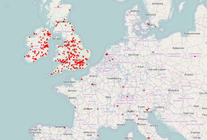
A screenshot of the results:

The above example uses OpenStreetMap for the tile images, but Leaflet lets you choose other services. For example, in the following screenshot the tiles are coming from MapBox.

You can see the interactive maps in action here:

Tiles from OpenStreetMap

Tiles from MapBox

Summary

In general there are many options for data visualisation in Python, but in terms of browser-based interaction, Javascript is also an interesting option, and the two languages can play well together. This article has shown that building a simple interactive map is a fairly straightforward process.

With a few lines of Python, we’ve been able to transform our data into a common format (GeoJSON) that can be passed onto Javascript for visualisation. Leaflet.js is a nice Javascript library that, almost out of the box, lets us create some nice interactive maps.

Tutorial Table of Contents:

Part 1: Collecting data
Part 2: Text Pre-processing
Part 3: Term Frequencies
Part 4: Rugby and Term Co-Occurrences
Part 5: Data Visualisation Basics
Part 6: Sentiment Analysis Basics
Part 7: Geolocation and Interactive Maps (this article)

@MarcoBonzanini

Functional Programming in Python

This is probably not the newest of the topics, but I haven’t had the chance to dig into it before, so here we go.

Python supports multiple programming paradigms, but it’s not best known for its Functional Programming style.
As its own creator has mentioned before, Python hasn’t been heavily influenced by other functional languages, but it does show some functional features. This is a very gentle introduction to Functional Programming in Python.

What is Functional Programming anyway?

Functional Programming is a programming paradigm based on the evaluation of expression, which avoids changing-state and mutable data. Popular functional languages include Lisp (and family), ML (and family), Haskell, Erlang and Clojure.

Functional Programming can be seen as a subset of Declarative Programming (as opposed to Imperative Programming).

Some of the characteristics of Functional Programming are:

Avoid state representation
Data are immutable
First class functions
High-order functions
Recursion

One of the key motivations beyond Functional Programming, and beyond some of its aspects like no changing-state and no mutable data, is the need to eliminate side effects, i.e. changes in the state that don’t really depend on the function input, making the program more difficult to understand and predict.

State representation and Transformation

In functional programming, functions transform input into output, without an intermediate representation of the current state.

Consider the following code:

def square(x):
    return x*x

input = [1, 2, 3, 4]
output = []
for v in input:
    output.append(square(v))

The code takes a list as input and iterates through its individual values applying the function square() to them; the final outcome is stored in the variable output which is initially an empty list, and is updated during the iteration.

Now, let’s consider the following functional style:

def square(x):
    return x*x

input = [1, 2, 3, 4]
output = map(square, input)

The logic is very similar: apply the function square() to all the element of the list given as input, but there is no internal state representation. The output is also a little bit different, as the map() function will return an iterator rather than a list.

Data are immutable

Related to the point above, the concept of immutable data can be summarised as: functions will return new data as the outcome of a computation, leaving the original input intact.

As mentioned earlier, Python is not a purely functional language, so there are both mutable and immutable data structures, e.g. lists are mutable arrays, while tuples are immutable:

>>> mutable = [1, 2, 3, 4]
>>> mutable[0] = 100
>>> mutable
[100, 2, 3, 4]
>>> mutable.append('hello')
>>> mutable
[100, 2, 3, 4, 'hello']

>>> immutable = (1, 2, 3, 4)
>>> immutable[0] = 100
Traceback (most recent call last):
  File "<stdin>", line 1, in <module>
TypeError: 'tuple' object does not support item assignment
>>> immutable.append('hello')
Traceback (most recent call last):
  File "<stdin>", line 1, in <module>
AttributeError: 'tuple' object has no attribute 'append'
>>> immutable
(1, 2, 3, 4)

First class functions and High-order functions

Functions being first class means that they can appear anywhere in a program, including return values and arguments of other functions. For example:

def greet(name):
    print("Hello %s!" % name)

say_hello = greet
say_hello('World')
# Hello World!

High-order functions are functions which can take functions as arguments (or return them as results). For example, this is what the map() function does, as one of the arguments is the name of the function to apply to a sequence. Notice the difference between the following two lines:

# some_func is an input of other_func()
out = other_func(some_func, some_data)
# the output of some_func() is the input of other_func()
out = other_func(some_func(some_data))

The first case represents a high-order function.

Recursion

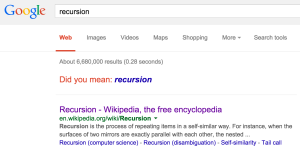
“To understand recursion, you must understand recursion.”

A recursive function calls itself on a smaller input, until the problem is reduced to some base case. For example, the factorial can be calculated in Python as:

def factorial(n):
    if n == 0:
        return 1
    else:
        return n * factorial(n-1)

Recursion is also a way to achieve iteration, usually in a more compact and elegant way, again without using internal state representation and without modifying the input data.

While it is possible to write recursive functions in Python, its interpreter doesn’t recognise tail recursion, an optimisation technique typically used by functional languages.

What else?

Besides the already mentioned map() function, there is more Functional Programming support in the Python standard library.

reduce() and filter()

The functions reduce() and filter() naturally belong together with the map() function. While map will apply a function over a sequence, producing a sequence as output, reduce will apply a function of two arguments cumulatively to the items in a sequence, in order to reduce the sequence to a single value.

In Python 3, reduce() is not a core built-infunction anymore and it has been moved to functools (still part of the standard library), i.e. in order to use it you need to import it as follows:

from functools import reduce

The use of filter() consists in applying a function to each item in a sequence, building a new sequence for those items that return true. For example:

def is_odd(n):
   return n%2 == 1
 
print(is_odd(2))
# False
print(is_odd(3))
# True
values = [1, 2, 3, 4, 5, 6]
result = filter(is_odd, values)
print(list(result))
# [1, 3, 5]

Notice: the term sequence has to be intended as iterable, and for both map() and filter() the return type is a generator (hence the use of list() to visualise the actual list).

lambda functions

Python supports the definition of lambda functions, i.e. small anonymous functions not necessarily bound to a name, at runtime. The use of anonymous functions is fairly common in Functional Programming, and it’s easy to see their use related to map/reduce/filter:

words = "The quick brown fox".split()
words_len = map(lambda w: len(w), words)
print(words)
# ['The', 'quick', 'brown', 'fox']
print(list(words_len))
# [3, 5, 5, 3]

Notice: the short lambda function above is just an example, in this case we could use len() directly.

itertools

The itertools module groups a number of functions related to iterators and their use/combination. Most of the basic and not-so-basic functionality that you might need to deal with iterators are already implemented there. The official Python documentation has a nice tutorial on Functional Programming, where the itertools module is described in details.

Generators for lazy-evaluation

Generator functions and generator expressions in Python provide objects that behave like an iterator (i.e. they can be looped over), without having the full content of the iterable loaded in memory. This concept is linked to lazy-evaluation, i.e. a call-by-need strategy where an item in a sequence is evaluated only when it’s needed, otherwise it’s not loaded in memory. This has repercussions on the amount of memory needed to deal with large sequences.

Some Final Thoughts

The topic of Functional Programming deserves definitely more than a blog post.

While Functional Programming has its benefits, Python is not a pure functional language. In particular, the mix of mutable and immutable data structures makes it difficult to truly separate the functional aspects of the language from the non-functional ones. The lack of some optimisations (e.g. no tail recursion) also makes some aspects of Functional Programming particularly costly, raising some questions about efficiency.

Even though Python is not openly inspired by other functional language, I think it’s always important to have an open mind regarding different programming paradigms. From this point of view, knowing what Python can (and can’t) do and how can only be beneficial for any Python user.

Please leave a comment or share if you liked (or disliked!) the article.

@MarcoBonzanini

Mining Twitter Data with Python (Part 6 – Sentiment Analysis Basics)

Sentiment Analysis is one of the interesting applications of text analytics. Although the term is often associated with sentiment classification of documents, broadly speaking it refers to the use of text analytics approaches applied to the set of problems related to identifying and extracting subjective material in text sources.

This article continues the series on mining Twitter data with Python, describing a simple approach for Sentiment Analysis and applying it to the rubgy data set (see Part 4).

Tutorial Table of Contents:

Part 1: Collecting data
Part 2: Text Pre-processing
Part 3: Term Frequencies
Part 4: Rugby and Term Co-Occurrences
Part 5: Data Visualisation Basics
Part 6: Sentiment Analysis Basics (this article)
Part 7: Geolocation and Interactive Maps

A Simple Approach for Sentiment Analysis

The technique we’re discussing in this post has been elaborated from the traditional approach proposed by Peter Turney in his paper Thumbs Up or Thumbs Down? Semantic Orientation Applied to Unsupervised Classification of Reviews. A lot of work has been done in Sentiment Analysis since then, but the approach has still an interesting educational value. In particular, it is intuitive, simple to understand and to test, and most of all unsupervised, so it doesn’t require any labelled data for training.

Firstly, we define the Semantic Orientation (SO) of a word as the difference between its associations with positive and negative words. In practice, we want to calculate “how close” a word is with terms like good and bad. The chosen measure of “closeness” is Pointwise Mutual Information (PMI), calculated as follows (t1 and t2 are terms):

$\mbox{PMI}(t_1, t_2) = \log\Bigl(\frac{P(t_1 \wedge t_2)}{P(t_1) \cdot P(t_2)}\Bigr)$

In Turney’s paper, the SO of a word was calculated against excellent and poor, but of course we can extend the vocabulary of positive and negative terms. Using $V^{+}$ and a vocabulary of positive terms and $V^{-}$ for the negative ones, the Semantic Orientation of a term t is hence defined as:

$\mbox{SO}(t) = \sum_{t' \in V^{+}}\mbox{PMI}(t, t') - \sum_{t' \in V^{-}}\mbox{PMI}(t, t')$

We can build our own list of positive and negative terms, or we can use one of the many resources available on-line, for example the opinion lexicon by Bing Liu.

Computing Term Probabilities

In order to compute $P(t)$ (the probability of observing the term t) and $P(t_1 \wedge t_2)$ (the probability of observing the terms t1 and t2 occurring together) we can re-use some previous code to calculate term frequencies and term co-occurrences. Given the set of documents (tweets) D, we define the Document Frequency (DF) of a term as the number of documents where the term occurs. The same definition can be applied to co-occurrent terms. Hence, we can define our probabilities as:

$P(t) = \frac{\mbox{DF}(t)}{|D|}\\ P(t_1 \wedge t_2) = \frac{\mbox{DF}(t_1 \wedge t_2)}{|D|}$

In the previous articles, the document frequency for single terms was stored in the dictionaries count_single and count_stop_single (the latter doesn’t store stop-words), while the document frequency for the co-occurrencies was stored in the co-occurrence matrix com

This is how we can compute the probabilities:

# n_docs is the total n. of tweets
p_t = {}
p_t_com = defaultdict(lambda : defaultdict(int))

for term, n in count_stop_single.items():
    p_t[term] = n / n_docs
    for t2 in com[term]:
        p_t_com[term][t2] = com[term][t2] / n_docs

Computing the Semantic Orientation

Given two vocabularies for positive and negative terms:

positive_vocab = [
    'good', 'nice', 'great', 'awesome', 'outstanding',
    'fantastic', 'terrific', ':)', ':-)', 'like', 'love',
    # shall we also include game-specific terms?
    # 'triumph', 'triumphal', 'triumphant', 'victory', etc.
]
negative_vocab = [
    'bad', 'terrible', 'crap', 'useless', 'hate', ':(', ':-(',
    # 'defeat', etc.
]

We can compute the PMI of each pair of terms, and then compute the
Semantic Orientation as described above:

pmi = defaultdict(lambda : defaultdict(int))
for t1 in p_t:
    for t2 in com[t1]:
        denom = p_t[t1] * p_t[t2]
        pmi[t1][t2] = math.log2(p_t_com[t1][t2] / denom)

semantic_orientation = {}
for term, n in p_t.items():
    positive_assoc = sum(pmi[term][tx] for tx in positive_vocab)
    negative_assoc = sum(pmi[term][tx] for tx in negative_vocab)
    semantic_orientation[term] = positive_assoc - negative_assoc

The Semantic Orientation of a term will have a positive (negative) value if the term is often associated with terms in the positive (negative) vocabulary. The value will be zero for neutral terms, e.g. the PMI’s for positive and negative balance out, or more likely a term is never observed together with other terms in the positive/negative vocabularies.

We can print out the semantic orientation for some terms:

semantic_sorted = sorted(semantic_orientation.items(), 
                         key=operator.itemgetter(1), 
                         reverse=True)
top_pos = semantic_sorted[:10]
top_neg = semantic_sorted[-10:]

print(top_pos)
print(top_neg)
print("ITA v WAL: %f" % semantic_orientation['#itavwal'])
print("SCO v IRE: %f" % semantic_orientation['#scovire'])
print("ENG v FRA: %f" % semantic_orientation['#engvfra'])
print("#ITA: %f" % semantic_orientation['#ita'])
print("#FRA: %f" % semantic_orientation['#fra'])
print("#SCO: %f" % semantic_orientation['#sco'])
print("#ENG: %f" % semantic_orientation['#eng'])
print("#WAL: %f" % semantic_orientation['#wal'])
print("#IRE: %f" % semantic_orientation['#ire'])

Different vocabularies will produce different scores. Using the opinion lexicon from Bing Liu, this is what we can observed on the Rugby data-set:

# the top positive terms
[('fantastic', 91.39950482011552), ('@dai_bach', 90.48767241244532), ('hoping', 80.50247748725415), ('#it', 71.28333427277785), ('days', 67.4394844955977), ('@nigelrefowens', 64.86112716005566), ('afternoon', 64.05064208341855), ('breathtaking', 62.86591435212975), ('#wal', 60.07283361352875), ('annual', 58.95378954406133)]
# the top negative terms
[('#england', -74.83306534609066), ('6', -76.0687215594536), ('#itavwal', -78.4558633116863), ('@rbs_6_nations', -80.89363516601993), ("can't", -81.75379628180468), ('like', -83.9319149443813), ('10', -85.93073078165587), ('italy', -86.94465165178258), ('#engvfra', -113.26188957010228), ('ball', -161.82146824640125)]
# Matches
ITA v WAL: -78.455863
SCO v IRE: -73.487661
ENG v FRA: -113.261890
# Individual team
#ITA: 53.033824
#FRA: 14.099372
#SCO: 4.426723
#ENG: -0.462845
#WAL: 60.072834
#IRE: 19.231722

Some Limitations

The PMI-based approach has been introduced as simple and intuitive, but of course it has some limitations. The semantic scores are calculated on terms, meaning that there is no notion of “entity” or “concept” or “event”. For example, it would be nice to aggregate and normalise all the references to the team names, e.g. #ita, Italy and Italia should all contribute to the semantic orientation of the same entity. Moreover, do the opinions on the individual teams also contribute to the overall opinion on a match?

Some aspects of natural language are also not captured by this approach, more notably modifiers and negation: how do we deal with phrases like not bad (this is the opposite of just bad) or very good (this is stronger than just good)?

Summary

This article has continued the tutorial on mining Twitter data with Python introducing a simple approach for Sentiment Analysis, based on the computation of a semantic orientation score which tells us whether a term is more closely related to a positive or negative vocabulary. The intuition behind this approach is fairly simple, and it can be implemented using Pointwise Mutual Information as a measure of association. The approach has of course some limitations, but it’s a good starting point to get familiar with Sentiment Analysis.

@MarcoBonzanini

Part 1: Collecting data
Part 2: Text Pre-processing
Part 3: Term Frequencies
Part 4: Rugby and Term Co-Occurrences
Part 5: Data Visualisation Basics
Part 6: Sentiment Analysis Basics (this article)
Part 7: Geolocation and Interactive Maps

Getting started with Neo4j and Python

This article is a brief introduction to Neo4j, one of the most popular graph databases, and its integration with Python.

Graph Databases

Graph databases are a family of NoSQL databases, based on the concept of modelling your data as a graph, i.e. a collection of nodes (representing entities) and edges (representing relationships).

The motivation behind the use of a graph database is the need to model small records which are deeply interconnected, forming a complex web that is difficult to represent in a relational fashion. Graph databases are particularly good at supporting queries that actually make use of such connections, i.e. by traversing the graph. Examples of suitable applications include social networks, recommendation engines (e.g. “show me movies that my best friends like”) and many other cases of link-rich domains.

Quick Installation

From the Neo4j web-site, we can download the community edition of Neo4j. At the moment of this writing, the last version is 2.2.0, which provides improved performance and a re-design of the UI. To install the software, simply unzip it:

tar zxf neo4j-community-2.2.0-unix.tar.gz
ln -s neo4j-community-2.2.0 neo4j

We can immediately run the server:

cd neo4j
./bin/neo4j start

and now we can point the browser to http://localhost:7474 for a nice web GUI. The first time you open the interface, you’ll be asked to set a password for the user “neo4j”.

If you want to stop the server, you can type:

./bin/neo4j stop

Interfacing with Python

There is no shortage of Neo4j clients available for several programming languages, including Python. An interesting project, which makes use of the Neo4j REST interface, is Neo4jRestClient. Quick installation:

pip install neo4jrestclient

All the features of this client are listed in the docs.

Creating a sample graph

Let’s start with a simple social-network-like application, where users know each others and like different “things”. In this example, users and things will be nodes in our database. Each node can be associated with labels, used to describe the type of node. The following code will create two nodes labelled as User and two nodes labelled as Beer:

from neo4jrestclient.client import GraphDatabase

db = GraphDatabase("http://localhost:7474", username="neo4j", password="mypassword")

# Create some nodes with labels
user = db.labels.create("User")
u1 = db.nodes.create(name="Marco")
user.add(u1)
u2 = db.nodes.create(name="Daniela")
user.add(u2)

beer = db.labels.create("Beer")
b1 = db.nodes.create(name="Punk IPA")
b2 = db.nodes.create(name="Hoegaarden Rosee")
# You can associate a label with many nodes in one go
beer.add(b1, b2)

The second step is all about connecting the dots, which in graph DB terminology means creating the relationships.

# User-likes-&amp;gt;Beer relationships
u1.relationships.create("likes", b1)
u1.relationships.create("likes", b2)
u2.relationships.create("likes", b1)
# Bi-directional relationship?
u1.relationships.create("friends", u2)

We notice that relationships have a direction, so we can easily model subject-predicate-object kind of relationships. In case we need to model bi-directional relationship, like in a friend-of link in a social network, there are essentially two options:

Add two edge per relationship, one for each direction
Add one edge per relationship, with an arbitrary direction, and then ignoring the direction in the query

In this example, we’re following the second option.

Querying the graph

The Neo4j Browser available at http://localhost:7474/ provides a nice way to query the DB and visualise the results, both as a list of record and in a visual form.

The query language for Neo4j is called Cypher. It allows to describe patterns in graphs, in a declarative fashion, i.e. just like SQL, you describe what you want, rather then how to retrieve it. Cypher uses some sort of ASCII-art to describe nodes, relationships and their direction.

For example, we can retrieve our whole graph using the following Cypher query:

MATCH (n)-[r]-&amp;gt;(m) RETURN n, r, m;

And the outcome in the browser:

In plain English, what the query is trying to match is “any node n, linked to a node m via a relationship r“. Suggestion: with a huge graph, use a LIMIT clause.

Of course we can also embed Cypher in our Python app, for example:

from neo4jrestclient import client

q = 'MATCH (u:User)-[r:likes]-&amp;gt;(m:Beer) WHERE u.name="Marco" RETURN u, type(r), m'
# "db" as defined above
results = db.query(q, returns=(client.Node, str, client.Node))
for r in results:
    print("(%s)-[%s]-&amp;gt;(%s)" % (r[0]["name"], r[1], r[2]["name"]))
# The output:
# (Marco)-[likes]-&amp;gt;(Punk IPA)
# (Marco)-[likes]-&amp;gt;(Hoegaarden Rosee)

The above query will retrieve all the triplets User-likes-Beer for the user Marco. The results variable will be a list of tuples, matching the format that we gave in Cypher with the RETURN keyword.

Summary

Graph databases, one of the NoSQL flavours, provide an interesting way to model data with rich interconnections. Examples of applications that are particularly suitable for graph databases are social networks and recommendation systems. This article has introduced Neo4j, one of the main examples of Graph DB, and its use with Python using the Neo4j REST client. We have seen how to create nodes and relationships, and how to query the graph using Cypher, the Neo4j query language.