Mining Twitter Data with Python: Part 5 – Data Visualisation Basics

A picture is worth a thousand tweets: more often than not, designing a good visual representation of our data, can help us make sense of them and highlight interesting insights. After collecting and analysing Twitter data, the tutorial continues with some notions on data visualisation with Python.

Tutorial Table of Contents:

From Python to Javascript with Vincent

While there are some options to create plots in Python using libraries like matplotlib or ggplot, one of the coolest libraries for data visualisation is probably D3.js which is, as the name suggests, based on Javascript. D3 plays well with web standards like CSS and SVG, and allows to create some wonderful interactive visualisations.

Vincent bridges the gap between a Python back-end and a front-end that supports D3.js visualisation, allowing us to benefit from both sides. The tagline of Vincent is in fact “The data capabilities of Python. The visualization capabilities of JavaScript”. Vincent, a Python library, takes our data in Python format and translates them into Vega, a JSON-based visualisation grammar that will be used on top of D3. It sounds quite complicated, but it’s fairly simple and pythonic. You don’t have to write a line in Javascript/D3 if you don’t want to.

Firstly, let’s install Vincent:

pip install vincent

Secondly, let’s create our first plot. Using the list of most frequent terms (without hashtags) from our rugby data set, we want to plot their frequencies:

import vincent

word_freq = count_terms_only.most_common(20)
labels, freq = zip(*word_freq)
data = {'data': freq, 'x': labels}
bar = vincent.Bar(data, iter_idx='x')
bar.to_json('term_freq.json')

At this point, the file term_freq.json will contain a description of the plot that can be handed over to D3.js and Vega. A simple template (taken from Vincent resources) to visualise the plot:

<html>
<head>
    <title>Vega Scaffold</title>
    <script src="http://d3js.org/d3.v3.min.js" charset="utf-8"></script>
    <script src="http://d3js.org/topojson.v1.min.js"></script>
    <script src="http://d3js.org/d3.geo.projection.v0.min.js" charset="utf-8"></script>
    <script src="http://trifacta.github.com/vega/vega.js"></script>
</head>
<body>
    <div id="vis"></div>
</body>
<script type="text/javascript">
// parse a spec and create a visualization view
function parse(spec) {
  vg.parse.spec(spec, function(chart) { chart({el:"#vis"}).update(); });
}
parse("term_freq.json");
</script>
</html>

Save the above HTML page as chart.html and run the simple Python web server:

python -m http.server 8888 # Python 3
python -m SimpleHTTPServer 8888 # Python 2

Now you can open your browser at http://localhost:8888/chart.html and observe the result:
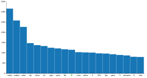
Term Frequencies

Notice: you could save the HTML template directly from Python with:

bar.to_json('term_freq.json', html_out=True, html_path='chart.html')

but, at least in Python 3, the output is not a well formed HTML and you’d need to manually strip some characters.

With this procedure, we can plot many different types of charts with Vincent. Let’s take a moment to browse the docs and see its capabilities.

Time Series Visualisation

Another interesting aspect of analysing data from Twitter is the possibility to observe the distribution of tweets over time. In other words, if we organise the frequencies into temporal buckets, we could observe how Twitter users react to real-time events.

One of my favourite tools for data analysis with Python is Pandas, which also has a fairly decent support for time series. As an example, let’s track the hashtag #ITAvWAL to observe what happened during the first match.

Firstly, if we haven’t done it yet, we need to install Pandas:

pip install pandas

In the main loop which reads all the tweets, we simply track the occurrences of the hashtag, i.e. we can refactor the code from the previous episodes into something similar to:

import pandas
import json

dates_ITAvWAL = []
# f is the file pointer to the JSON data set
for line in f:
    tweet = json.loads(line)
    # let's focus on hashtags only at the moment
    terms_hash = [term for term in preprocess(tweet['text']) if term.startswith('#')]
    # track when the hashtag is mentioned
    if '#itavwal' in terms_hash:
        dates_ITAvWAL.append(tweet['created_at'])

# a list of "1" to count the hashtags
ones = [1]*len(dates_ITAvWAL)
# the index of the series
idx = pandas.DatetimeIndex(dates_ITAvWAL)
# the actual series (at series of 1s for the moment)
ITAvWAL = pandas.Series(ones, index=idx)

# Resampling / bucketing
per_minute = ITAvWAL.resample('1Min', how='sum').fillna(0)

The last line is what allows us to track the frequencies over time. The series is re-sampled with intervals of 1 minute. This means all the tweets falling within a particular minute will be aggregated, more precisely they will be summed up, given how='sum'. The time index will not keep track of the seconds anymore. If there is no tweet in a particular minute, the fillna() function will fill the blanks with zeros.

To put the time series in a plot with Vincent:

time_chart = vincent.Line(ITAvWAL)
time_chart.axis_titles(x='Time', y='Freq')
time_chart.to_json('time_chart.json')

Once you embed the time_chart.json file into the HTML template discussed above, you’ll see this output:
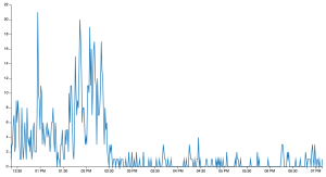
Time Series

The interesting moments of the match are observable from the spikes in the series. The first spike just before 1pm corresponds to the first Italian try. All the other spikes between 1:30 and 2:30pm correspond to Welsh tries and show the Welsh dominance during the second half. The match was over by 2:30, so after that Twitter went quiet.

Rather than just observing one sequence at a time, we could compare different series to observe how the matches has evolved. So let’s refactor the code for the time series, keeping track of the three different hashtags #ITAvWAL, #SCOvIRE and #ENGvFRA into the corresponding pandas.Series.

# all the data together
match_data = dict(ITAvWAL=per_minute_i, SCOvIRE=per_minute_s, ENGvFRA=per_minute_e)
# we need a DataFrame, to accommodate multiple series
all_matches = pandas.DataFrame(data=match_data,
                               index=per_minute_i.index)
# Resampling as above
all_matches = all_matches.resample('1Min', how='sum').fillna(0)

# and now the plotting
time_chart = vincent.Line(all_matches[['ITAvWAL', 'SCOvIRE', 'ENGvFRA']])
time_chart.axis_titles(x='Time', y='Freq')
time_chart.legend(title='Matches')
time_chart.to_json('time_chart.json')

And the output:
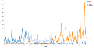
time2

We can immediately observe when the different matches took place (approx 12:30-2:30, 2:30-4:30 and 5-7) and we can see how the last match had the all the attentions, especially in the end when the winner was revealed.

Summary

Data visualisation is an important discipline in the bigger context of data analysis. By supporting visual representations of our data, we can provide interesting insights. We have discussed a relatively simple option to support data visualisation with Python using Vincent. In particular, we have seen how we can easily bridge the gap between Python and a language like Javascript that offers a great tool like D3.js, one of the most important libraries for interactive visualisation. Overall, we have just scratched the surface of data visualisation, but as a starting point this should be enough to get some nice ideas going. The nature of Twitter as a medium has also encouraged a quick look into the topic of time series analysis, allowing us to mention pandas as a great Python tool.

If this article has given you some ideas for data visualisation, please leave a comment below or get in touch.

@MarcoBonzanini

Tutorial Table of Contents:

Mining Twitter Data with Python (Part 4: Rugby and Term Co-occurrences)

Last Saturday was the closing day of the Six Nations Championship, an annual international rugby competition. Before turning on the TV to watch Italy being trashed by Wales, I decided to use this event to collect some data from Twitter and perform some exploratory text analysis on something more interesting than the small list of my tweets.

This article continues the tutorial on Twitter Data Mining, re-using what we discussed in the previous articles with some more realistic data. It also expands the analysis by introducing the concept of term co-occurrence.

Tutorial Table of Contents:

The Application Domain

As the name suggests, six teams are involved in the competition: England, Ireland, Wales, Scotland, France and Italy. This means that we can expect the event to be tweeted in multiple languages (English, French, Italian, Welsh, Gaelic, possibly other languages as well), with English being the major language. Assuming the team names will be mentioned frequently, we could decide to look also for their nicknames, e.g. Les Bleus for France or Azzurri for Italy. During the last day of the competition, three matches are played sequentially. Three teams in particular had a shot for the title: England, Ireland and Wales. At the end, Ireland won the competition but everything was open until the very last minute.

Setting Up

I used the streaming API to download all the tweets containing the string #rbs6nations during the day. Obviously not all the tweets about the event contained the hashtag, but this is a good baseline. The time frame for the download was from around 12:15PM to 7:15PM GMT, that is from about 15 minutes before the first match, to about 15 minutes after the last match was over. At the end, more than 18,000 tweets have been downloaded in JSON format, making for about 75Mb of data. This should be small enough to quickly do some processing in memory, and at the same time big enough to observe something possibly interesting.

The textual content of the tweets has been pre-processed with tokenisation and lowercasing using the preprocess() function introduced in Part 2 of the tutorial.

Interesting terms and hashtags

Following what we discussed in Part 3 (Term Frequencies), we want to observe the most common terms and hashtags used during day. If you have followed the discussion about creating different lists of tokens in order to capture terms without hashtags, hashtags only, removing stop-words, etc. you can play around with the different lists.

This is the unsurprising list of top 10 most frequent terms (terms_only in Part 3) in the data set.

[('ireland', 3163), ('england', 2584), ('wales', 2271), ('…', 2068), ('day', 1479), ('france', 1380), ('win', 1338), ('rugby', 1253), ('points', 1221), ('title', 1180)]

The first three terms correspond to the teams who had a go for the title. The frequencies also respect the order in the final table. The fourth term is instead a punctuation mark that we missed and didn’t include in the list of stop-words. This is because string.punctuation only contains ASCII symbols, while here we’re dealing with a unicode character. If we dig into the data, there will be more examples like this, but for the moment we don’t worry about it.

After adding the suspension-points symbol to the list of stop-words, we have a new entry at the end of the list:

[('ireland', 3163), ('england', 2584), ('wales', 2271), ('day', 1479), ('france', 1380), ('win', 1338), ('rugby', 1253), ('points', 1221), ('title', 1180), ('🍀', 1154)]

Interestingly, a new token we didn’t account for, an Emoji symbol (in this case, the Irish Shamrock).

If we have a look at the most common hashtags, we need to consider that #rbs6nations will be by far the most common token (that’s our search term for downloading the tweets), so we can exclude it from the list. This leave us with:

[('#engvfra', 1701), ('#itavwal', 927), ('#rugby', 880), ('#scovire', 692), ('#ireland', 686), ('#angfra', 554), ('#xvdefrance', 508), ('#crunch', 500), ('#wales', 446), ('#england', 406)]

We can observe that the most common hashtags, a part from #rugby, are related to the individual matches. In particular England v France has received the highest number of mentions, probably being the last match of the day with a dramatic finale. Something interesting to notice is that a fair amount of tweets also contained terms in French: the count for #angfra should in fact be added to #engvfra. Those unfamiliar with rugby probably wouldn’t recognise that also #crunch should be included with #EngvFra match, as Le Crunch is the traditional name for this event. So by far, the last match has received a lot of attention.

Term co-occurrences

Sometimes we are interested in the terms that occur together. This is mainly because the context gives us a better insight about the meaning of a term, supporting applications such as word disambiguation or semantic similarity. We discussed the option of using bigrams in the previous article, but we want to extend the context of a term to the whole tweet.

We can refactor the code from the previous article in order to capture the co-occurrences. We build a co-occurrence matrix com such that com[x][y] contains the number of times the term x has been seen in the same tweet as the term y:

from collections import defaultdict
# remember to include the other import from the previous post

com = defaultdict(lambda : defaultdict(int))

# f is the file pointer to the JSON data set
for line in f: 
    tweet = json.loads(line)
    terms_only = [term for term in preprocess(tweet['text']) 
                  if term not in stop 
                  and not term.startswith(('#', '@'))]

    # Build co-occurrence matrix
    for i in range(len(terms_only)-1):            
        for j in range(i+1, len(terms_only)):
            w1, w2 = sorted([terms_only[i], terms_only[j]])                
            if w1 != w2:
                com[w1][w2] += 1

While building the co-occurrence matrix, we don’t want to count the same term pair twice, e.g. com[A][B] == com[B][A], so the inner for loop starts from i+1 in order to build a triangular matrix, while sorted will preserve the alphabetical order of the terms.

For each term, we then extract the 5 most frequent co-occurrent terms, creating a list of tuples in the form ((term1, term2), count):

com_max = []
# For each term, look for the most common co-occurrent terms
for t1 in com:
    t1_max_terms = sorted(com[t1].items(), key=operator.itemgetter(1), reverse=True)[:5]
    for t2, t2_count in t1_max_terms:
        com_max.append(((t1, t2), t2_count))
# Get the most frequent co-occurrences
terms_max = sorted(com_max, key=operator.itemgetter(1), reverse=True)
print(terms_max[:5])

The results:

[(('6', 'nations'), 845), (('champions', 'ireland'), 760), (('nations', 'rbs'), 742), (('day', 'ireland'), 731), (('ireland', 'wales'), 674)]

This implementation is pretty straightforward, but depending on the data set and on the use of the matrix, one might want to look into tools like scipy.sparse for building a sparse matrix.

We could also look for a specific term and extract its most frequent co-occurrences. We simply need to modify the main loop including an extra counter, for example:

search_word = sys.argv[1] # pass a term as a command-line argument
count_search = Counter()
for line in f:
    tweet = json.loads(line)
    terms_only = [term for term in preprocess(tweet['text']) 
                  if term not in stop 
                  and not term.startswith(('#', '@'))]
    if search_word in terms_only:
        count_search.update(terms_only)
print("Co-occurrence for %s:" % search_word)
print(count_search.most_common(20))

The outcome for “ireland”:

[('champions', 756), ('day', 727), ('nations', 659), ('wales', 654), ('2015', 638), ('6', 613), ('rbs', 585), ('http://t.co/y0nvsvayln', 559), ('🍀', 526), ('10', 522), ('win', 377), ('england', 377), ('twickenham', 361), ('40', 360), ('points', 356), ('sco', 355), ('ire', 355), ('title', 346), ('scotland', 301), ('turn', 295)]

The outcome for “rugby”:

[('day', 476), ('game', 160), ('ireland', 143), ('england', 132), ('great', 105), ('today', 104), ('best', 97), ('well', 90), ('ever', 89), ('incredible', 87), ('amazing', 84), ('done', 82), ('amp', 71), ('games', 66), ('points', 64), ('monumental', 58), ('strap', 56), ('world', 55), ('team', 55), ('http://t.co/bhmeorr19i', 53)]

Overall, quite interesting.

Summary

This article has discussed a toy example of Text Mining on Twitter, using some realistic data taken during a sport event. Using what we have learnt in the previous episodes, we have downloaded some data using the streaming API, pre-processed the data in JSON format and extracted some interesting terms and hashtags from the tweets. The article has also introduced the concept of term co-occurrence, shown how to build a co-occurrence matrix and discussed how to use it to find some interesting insight.

@MarcoBonzanini

Mining Twitter Data with Python (Part 3: Term Frequencies)

This is the third part in a series of articles about data mining on Twitter. After collecting data and pre-processing some text, we are ready for some basic analysis. In this article, we’ll discuss the analysis of term frequencies to extract meaningful terms from our tweets.

Tutorial Table of Contents:

Counting Terms

Assuming we have collected a list of tweets (see Part 1 of the tutorial), the first exploratory analysis that we can perform is a simple word count. In this way, we can observe what are the terms most commonly used in the data set. In this example, I’ll use the set of my tweets, so the most frequent words should correspond to the topics I discuss (not necessarily, but bear with be for a couple of paragraphs).

We can use a custom tokeniser to split the tweets into a list of terms. The following code uses the preprocess() function described in Part 2 of the tutorial, in order to capture Twitter-specific aspects of the text, such as #hashtags, @-mentions, emoticons and URLs. In order to keep track of the frequencies while we are processing the tweets, we can use collections.Counter() which internally is a dictionary (term: count) with some useful methods like most_common():

import operator 
import json
from collections import Counter

fname = 'mytweets.json'
with open(fname, 'r') as f:
    count_all = Counter()
    for line in f:
        tweet = json.loads(line)
        # Create a list with all the terms
        terms_all = [term for term in preprocess(tweet['text'])]
        # Update the counter
        count_all.update(terms_all)
    # Print the first 5 most frequent words
    print(count_all.most_common(5))

The above code will produce some unimpressive results:

[(':', 44), ('rt', 26), ('to', 26), ('and', 25), ('on', 22)]

As you can see, the most frequent words (or should I say, tokens), are not exactly meaningful.

Removing stop-words

In every language, some words are particularly common. While their use in the language is crucial, they don’t usually convey a particular meaning, especially if taken out of context. This is the case of articles, conjunctions, some adverbs, etc. which are commonly called stop-words. In the example above, we can see three common stop-words – to, and and on. Stop-word removal is one important step that should be considered during the pre-processing stages. One can build a custom list of stop-words, or use available lists (e.g. NLTK provides a simple list for English stop-words).

Given the nature of our data and our tokenisation, we should also be careful with all the punctuation marks and with terms like RT (used for re-tweets) and via (used to mention the original author of an article or a re-tweet), which are not in the default stop-word list.

from nltk.corpus import stopwords
import string

punctuation = list(string.punctuation)
stop = stopwords.words('english') + punctuation + ['rt', 'via']

We can now substitute the variable terms_all in the first example with something like:

terms_stop = [term for term in preprocess(tweet['text']) if term not in stop]

After counting, sorting the terms and printing the top 5, this is the result:

[('python', 11), ('@miguelmalvarez', 9), ('#python', 9), ('data', 8), ('@danielasfregola', 7)]

So apparently I mostly tweet about Python and data, and the users I re-tweet more often are @miguelmalvarez and @danielasfregola, it sounds about right.

More term filters

Besides stop-word removal, we can further customise the list of terms/tokens we are interested in. Here you have some examples that you can embed in the first fragment of code:

# Count terms only once, equivalent to Document Frequency
terms_single = set(terms_all)
# Count hashtags only
terms_hash = [term for term in preprocess(tweet['text']) 
              if term.startswith('#')]
# Count terms only (no hashtags, no mentions)
terms_only = [term for term in preprocess(tweet['text']) 
              if term not in stop and 
              not term.startswith(('#', '@'))] 
              # mind the ((double brackets))
              # startswith() takes a tuple (not a list) if 
              # we pass a list of inputs

After counting and sorting, these are my most commonly used hashtags:

[('#python', 9), ('#scala', 6), ('#nosql', 4), ('#bigdata', 3), ('#nlp', 3)]

and these are my most commonly used terms:

[('python', 11), ('data', 8), ('summarisation', 6), ('twitter', 5), ('nice', 5)]

“nice”?

While the other frequent terms represent a clear topic, more often than not simple term frequencies don’t give us a deep explanation of what the text is about. To put things in context, let’s consider sequences of two terms (a.k.a. bigrams).

from nltk import bigrams 

terms_bigram = bigrams(terms_stop)

The bigrams() function from NLTK will take a list of tokens and produce a list of tuples using adjacent tokens. Notice that we could use terms_all to compute the bigrams, but we would probably end up with a lot of garbage. In case we decide to analyse longer n-grams (sequences of n tokens), it could make sense to keep the stop-words, just in case we want to capture phrases like “to be or not to be”.

So after counting and sorting the bigrams, this is the result:

[(('nice', 'article'), 4), (('extractive', 'summarisation'), 4), (('summarisation', 'sentence'), 3), (('short', 'paper'), 3), (('paper', 'extractive'), 2)]

So apparently I tweet about nice articles (I wouldn’t bother sharing the boring ones) and extractive summarisation (the topic of my PhD dissertation). This also sounds about right.

Summary

This article has built on top of the previous ones to discuss some basis for extracting interesting terms from a data set of tweets, by using simple term frequencies, stop-word removal and n-grams. While these approaches are extremely simple to implement, they are quite useful to have a bird’s eye view on the data. We have used some components of NLTK (introduced in a previous article), so we don’t have to re-invent the wheel.

@MarcoBonzanini

Tutorial Table of Contents:

Mining Twitter Data with Python (Part 2: Text Pre-processing)

This is the second part of a series of articles about data mining on Twitter. In the previous episode, we have seen how to collect data from Twitter. In this post, we’ll discuss the structure of a tweet and we’ll start digging into the processing steps we need for some text analysis.

Table of Contents of this tutorial:

The Anatomy of a Tweet

Assuming that you have collected a number of tweets and stored them in JSON as suggested in the previous article, let’s have a look at the structure of a tweet:

import json

with open('mytweets.json', 'r') as f:
    line = f.readline() # read only the first tweet/line
    tweet = json.loads(line) # load it as Python dict
    print(json.dumps(tweet, indent=4)) # pretty-print

The key attributes are the following:

  • text: the text of the tweet itself
  • created_at: the date of creation
  • favorite_count, retweet_count: the number of favourites and retweets
  • favorited, retweeted: boolean stating whether the authenticated user (you) have favourited or retweeted this tweet
  • lang: acronym for the language (e.g. “en” for english)
  • id: the tweet identifier
  • place, coordinates, geo: geo-location information if available
  • user: the author’s full profile
  • entities: list of entities like URLs, @-mentions, hashtags and symbols
  • in_reply_to_user_id: user identifier if the tweet is a reply to a specific user
  • in_reply_to_status_id: status identifier id the tweet is a reply to a specific status

As you can see there’s a lot of information we can play with. All the *_id fields also have a *_id_str counterpart, where the same information is stored as a string rather than a big int (to avoid overflow problems). We can imagine how these data already allow for some interesting analysis: we can check who is most favourited/retweeted, who’s discussing with who, what are the most popular hashtags and so on. Most of the goodness we’re looking for, i.e. the content of a tweet, is anyway embedded in the text, and that’s where we’re starting our analysis.

We start our analysis by breaking the text down into words. Tokenisation is one of the most basic, yet most important, steps in text analysis. The purpose of tokenisation is to split a stream of text into smaller units called tokens, usually words or phrases. While this is a well understood problem with several out-of-the-box solutions from popular libraries, Twitter data pose some challenges because of the nature of the language.

How to Tokenise a Tweet Text

Let’s see an example, using the popular NLTK library to tokenise a fictitious tweet:

from nltk.tokenize import word_tokenize

tweet = 'RT @marcobonzanini: just an example! :D http://example.com #NLP'
print(word_tokenize(tweet))
# ['RT', '@', 'marcobonzanini', ':', 'just', 'an', 'example', '!', ':', 'D', 'http', ':', '//example.com', '#', 'NLP']

You will notice some peculiarities that are not captured by a general-purpose English tokeniser like the one from NLTK: @-mentions, emoticons, URLs and #hash-tags are not recognised as single tokens. The following code will propose a pre-processing chain that will consider these aspects of the language.

import re

emoticons_str = r"""
    (?:
        [:=;] # Eyes
        [oO\-]? # Nose (optional)
        [D\)\]\(\]/\\OpP] # Mouth
    )"""

regex_str = [
    emoticons_str,
    r'<[^>]+>', # HTML tags
    r'(?:@[\w_]+)', # @-mentions
    r"(?:\#+[\w_]+[\w\'_\-]*[\w_]+)", # hash-tags
    r'http[s]?://(?:[a-z]|[0-9]|[$-_@.&amp;+]|[!*\(\),]|(?:%[0-9a-f][0-9a-f]))+', # URLs

    r'(?:(?:\d+,?)+(?:\.?\d+)?)', # numbers
    r"(?:[a-z][a-z'\-_]+[a-z])", # words with - and '
    r'(?:[\w_]+)', # other words
    r'(?:\S)' # anything else
]
   
tokens_re = re.compile(r'('+'|'.join(regex_str)+')', re.VERBOSE | re.IGNORECASE)
emoticon_re = re.compile(r'^'+emoticons_str+'$', re.VERBOSE | re.IGNORECASE)

def tokenize(s):
    return tokens_re.findall(s)

def preprocess(s, lowercase=False):
    tokens = tokenize(s)
    if lowercase:
        tokens = [token if emoticon_re.search(token) else token.lower() for token in tokens]
    return tokens

tweet = 'RT @marcobonzanini: just an example! :D http://example.com #NLP'
print(preprocess(tweet))
# ['RT', '@marcobonzanini', ':', 'just', 'an', 'example', '!', ':D', 'http://example.com', '#NLP']

As you can see, @-mentions, emoticons, URLs and #hash-tags are now preserved as individual tokens.

If we want to process all our tweets, previously saved on file:

with open('mytweets.json', 'r') as f:
    for line in f:
        tweet = json.loads(line)
        tokens = preprocess(tweet['text'])
        do_something_else(tokens)

The tokeniser is probably far from perfect, but it gives you the general idea. The tokenisation is based on regular expressions (regexp), which is a common choice for this type of problem. Some particular types of tokens (e.g. phone numbers or chemical names) will not be captured, and will be probably broken into several tokens. To overcome this problem, as well as to improve the richness of your pre-processing pipeline, you can improve the regular expressions, or even employ more sophisticated techniques like Named Entity Recognition.

The core component of the tokeniser is the regex_str variable, which is a list of possible patterns. In particular, we try to capture some emoticons, HTML tags, Twitter @usernames (@-mentions), Twitter #hashtags, URLs, numbers, words with and without dashes and apostrophes, and finally “anything else”. Please take a moment to observe the regexp for capturing numbers: why don’t we just use \d+? The problem here is that numbers can appear in several different ways, e.g. 1000 can also be written as 1,000 or 1,000.00 — and we can get into more complications in a multi-lingual environment where commas and dots are inverted: “one thousand” can be written as 1.000 or 1.000,00 in many non-anglophone countries. The task of identifying numeric tokens correctly just gives you a glimpse of how difficult tokenisation can be.

The regular expressions are compiled with the flags re.VERBOSE, to allow spaces in the regexp to be ignored (see the multi-line emoticons regexp), and re.IGNORECASE to catch both upper and lowercases. The tokenize() function simply catches all the tokens in a string and returns them as a list. This function is used within preprocess(), which is used as a pre-processing chain: in this case we simply add a lowercasing feature for all the tokens that are not emoticons (e.g. :D doesn’t become :d).

Summary

In this article we have analysed the overall structure of a tweet, and we have discussed how to pre-process the text before we can get into some more interesting analysis. In particular, we have seen how tokenisation, despite being a well-understood problem, can get tricky with Twitter data. The proposed solution is far from perfect but it’s a good starting point, and fairly easy to extend.

@MarcoBonzanini

Table of Contents of this tutorial:

Mining Twitter Data with Python (Part 1: Collecting data)

Twitter is a popular social network where users can share short SMS-like messages called tweets. Users share thoughts, links and pictures on Twitter, journalists comment on live events, companies promote products and engage with customers. The list of different ways to use Twitter could be really long, and with 500 millions of tweets per day, there’s a lot of data to analyse and to play with.

This is the first in a series of articles dedicated to mining data on Twitter using Python. In this first part, we’ll see different options to collect data from Twitter. Once we have built a data set, in the next episodes we’ll discuss some interesting data applications.

Update July 2016: my new book on data mining for Social Media is out! Part of the content in this tutorial has been improved and expanded as part of the book, so please have a look. Chapter 2 about mining Twitter is available as a free sample from the publisher’s web site, and the companion code with many more examples is available on my GitHub

Table of Contents of this tutorial:

More updates: fixed version number of Tweepy to avoid problem with Python 3; fixed discussion on _json to get the JSON representation of a tweet; added example of process_or_store().

Register Your App

In order to have access to Twitter data programmatically, we need to create an app that interacts with the Twitter API.

The first step is the registration of your app. In particular, you need to point your browser to http://apps.twitter.com, log-in to Twitter (if you’re not already logged in) and register a new application. You can now choose a name and a description for your app (for example “Mining Demo” or similar). You will receive a consumer key and a consumer secret: these are application settings that should always be kept private. From the configuration page of your app, you can also require an access token and an access token secret. Similarly to the consumer keys, these strings must also be kept private: they provide the application access to Twitter on behalf of your account. The default permissions are read-only, which is all we need in our case, but if you decide to change your permission to provide writing features in your app, you must negotiate a new access token.

Important Note: there are rate limits in the use of the Twitter API, as well as limitations in case you want to provide a downloadable data-set, see:

Accessing the Data

Twitter provides REST APIs you can use to interact with their service. There is also a bunch of Python-based clients out there that we can use without re-inventing the wheel. In particular, Tweepy in one of the most interesting and straightforward to use, so let’s install it:

pip install tweepy==3.3.0

Update: the release 3.4.0 of Tweepy has introduced a problem with Python 3, currently fixed on github but not yet available with pip, for this reason we’re using version 3.3.0 until a new release is available.

More Updates: the release 3.5.0 of Tweepy, already available via pip, seems to solve the problem with Python 3 mentioned above.

In order to authorise our app to access Twitter on our behalf, we need to use the OAuth interface:

import tweepy
from tweepy import OAuthHandler

consumer_key = 'YOUR-CONSUMER-KEY'
consumer_secret = 'YOUR-CONSUMER-SECRET'
access_token = 'YOUR-ACCESS-TOKEN'
access_secret = 'YOUR-ACCESS-SECRET'

auth = OAuthHandler(consumer_key, consumer_secret)
auth.set_access_token(access_token, access_secret)

api = tweepy.API(auth)

The api variable is now our entry point for most of the operations we can perform with Twitter.

For example, we can read our own timeline (i.e. our Twitter homepage) with:

for status in tweepy.Cursor(api.home_timeline).items(10):
    # Process a single status
    print(status.text)

Tweepy provides the convenient Cursor interface to iterate through different types of objects. In the example above we’re using 10 to limit the number of tweets we’re reading, but we can of course access more. The status variable is an instance of the Status() class, a nice wrapper to access the data. The JSON response from the Twitter API is available in the attribute _json (with a leading underscore), which is not the raw JSON string, but a dictionary.

So the code above can be re-written to process/store the JSON:

for status in tweepy.Cursor(api.home_timeline).items(10):
    # Process a single status
    process_or_store(status._json)

What if we want to have a list of all our followers? There you go:

for friend in tweepy.Cursor(api.friends).items():
    process_or_store(friend._json)

And how about a list of all our tweets? Simple:

for tweet in tweepy.Cursor(api.user_timeline).items():
    process_or_store(tweet._json)

In this way we can easily collect tweets (and more) and store them in the original JSON format, fairly easy to convert into different data models depending on our storage (many NoSQL technologies provide some bulk import feature).

The function process_or_store() is a place-holder for your custom implementation. In the simplest form, you could just print out the JSON, one tweet per line:

def process_or_store(tweet):
    print(json.dumps(tweet))

Streaming

In case we want to “keep the connection open”, and gather all the upcoming tweets about a particular event, the streaming API is what we need. We need to extend the StreamListener() to customise the way we process the incoming data. A working example that gathers all the new tweets with the #python hashtag:

from tweepy import Stream
from tweepy.streaming import StreamListener

class MyListener(StreamListener):

    def on_data(self, data):
        try:
            with open('python.json', 'a') as f:
                f.write(data)
                return True
        except BaseException as e:
            print("Error on_data: %s" % str(e))
        return True

    def on_error(self, status):
        print(status)
        return True

twitter_stream = Stream(auth, MyListener())
twitter_stream.filter(track=['#python'])

Depending on the search term, we can gather tons of tweets within a few minutes. This is especially true for live events with a world-wide coverage (World Cups, Super Bowls, Academy Awards, you name it), so keep an eye on the JSON file to understand how fast it grows and consider how many tweets you might need for your tests. The above script will save each tweet on a new line, so you can use the command wc -l python.json from a Unix shell to know how many tweets you’ve gathered.

You can see a minimal working example of the Twitter Stream API in the following Gist:

twitter_stream_downloader.py

Summary

We have introduced tweepy as a tool to access Twitter data in a fairly easy way with Python. There are different types of data we can collect, with the obvious focus on the “tweet” object.

Once we have collected some data, the possibilities in terms of analytics applications are endless. In the next episodes, we’ll discuss some options.

@MarcoBonzanini

Table of Contents of this tutorial:

PyData London Meetup 2015-02-03

A quick update with my impressions on the last PyData London meet-up I attended this evening.

I missed the past couple of meet-ups because of some clash on my personal schedule, so this was my first time in the new venue, still close to Old Street, hosted by Lyst. A nice big room to accomodate many many people (more than 200 probably?), and a nice selection of craft beers.

We started with the usual initial community-related announcements, including the impressive achievement of the group: 1,000+ members on the meetup.com dedicated page! Well done guys!

The core topic of the evening was data visualisation. For this reason, the main candidate for Python Module Of The Month was (… drum roll …) matplotlib :-D

The first talk, “Thinking about data visualisation”, was given by Andy Kirk from Visualising Data. Thinking was an important keyword of the presentation: after an initial comparison between talent (e.g. artistic, creative) vs thinking, Andy went on discussing different aspects of thinking and how our thinking can provide more value to the visualisation we are proposing. Long story short, you don’t have to be an artist to create useful visualisation, assuming you take the context and the overall story into account.

The second talk, “Lies, damned lies and dataviz”, was given by Andrew Clegg from Etsy. Andrew started the presentation with some argument in support of providing good dataviz, and then he continued with a great sequence of examples of bad dataviz, discussing how some of them simply confuse the user without providing any additional insight, while others really trick the user into wrong conclusions. Whether these are damned lies or just bad design choices… well that’s another story.

Both presentations were really great, and both of them technology-agnostic, which is something I enjoyed for some reason.

During the final lightning-and-community-talks, the interesting news was the announcement of a new O’Reilly book on data visualisation with Python and Javascript (link to come).

Overall a very nice evening, congratulations to all the organisers.

PyData London meetup.com group:
http://www.meetup.com/PyData-London-Meetup/

Stemming, Lemmatisation and POS-tagging with Python and NLTK

This article describes some pre-processing steps that are commonly used in Information Retrieval (IR), Natural Language Processing (NLP) and text analytics applications.

In particular, the focus is on the comparison between stemming and lemmatisation, and the need for part-of-speech tagging in this context. The discussion shows some examples in NLTK, also as
Gist on github.

Stemming

Stemming is the process of reducing a word into its stem, i.e. its root form. The root form is not necessarily a word by itself, but it can be used to generate words by concatenating the right suffix.

For example, the words fish, fishes and fishing all stem into fish, which is a correct word. On the other side, the words study, studies and studying stems into studi, which is not an English word.

Most commonly, stemming algorithms (a.k.a. stemmers) are based on rules for suffix stripping.
The most famous example is the Porter stemmer, introduced in the 1980’s and currently implemented in a variety of programming languages.

Traditionally, search engines and other IR applications have applied stemming to improve the chance of matching different forms of a word, almost treating them like synonyms, as conceptually they “belong” together.

Lemmatisation

The purpose of Lemmatisation is to group together different inflected forms of a word, called lemma. The process is somehow similar to stemming, as it maps several words into one common root. The output of lemmatisation is a proper word, and basic suffix stripping wouldn’t provide the same outcome. For example, a lemmatiser should map gone, going and went into go. In order to achieve its purpose, lemmatisation requires to know about the context of a word, because the process relies on whether the word is a noun, a verb, etc.

Part-of-speech Tagging

Part-of-speech (POS) tagging is the process of assigning a word to its grammatical category, in order to understand its role within the sentence. Traditional parts of speech are nouns, verbs, adverbs, conjunctions, etc.

Part-of-speech taggers typically take a sequence of words (i.e. a sentence) as input, and provide a list of tuples as output, where each word is associated with the related tag.

Part-of-speech tagging is what provides the contextual information that a lemmatiser needs to choose the appropriate lemma.

Examples in Python and NLTK

One of the most popular packages for NLP in Python is the Natural Language Toolkit (NLTK). It includes several tools for text analytics, as well as training data for some of the tools, and also some well-known data sets.

To install NLTK:

pip install nltk

In order to install the additional data, you can use its internal tool. From a Python interactive shell, simply type:

import nltk
nltk.download()

This will open a GUI which you can use to choose which data you want to download (if you’re not using a GUI environment, the interface will be textual). In a dev environment, I normally just download all the data for all the packages in the default folder ($HOME/nltk_data) but you can personalise
your installation.

A full example of stemming, lemmatisation and POS-tagging is available as Gist on github.

Let’s focus on this snippet:

from nltk.stem import PorterStemmer, WordNetLemmatizer

stemmer = PorterStemmer()
lemmatiser = WordNetLemmatizer()

print("Stem %s: %s" % ("studying", stemmer.stem("studying")))
print("Lemmatise %s: %s" % ("studying", lemmatiser.lemmatize("studying")))
print("Lemmatise %s: %s" % ("studying", lemmatiser.lemmatize("studying", pos="v")))

The output will be:

Stem studying: studi
Lemmatise studying: studying
Lemmatise studying: study

We can observe that the stemming process doesn’t generate a real word, but a root form.
On the other side, the lemmatiser generates real words, but without contextual information it’s not able to distinguish between nouns and verbs, hence the lemmatisation process doesn’t change
the word. The context is provided by the POS tag (“v” for verb in this example).

In order to generate POS tags automatically, nltk comes with a simple function. The snippet for POS tagging:

from nltk import pos_tag
from nltk.tokenize import word_tokenize

s = "This is a simple sentence"
tokens = word_tokenize(s) # Generate list of tokens
tokens_pos = pos_tag(tokens) 

print(tokens_pos)

and the output will be:

[('This', 'DT'), ('is', 'VBZ'), ('a', 'DT'), ('simple', 'JJ'), ('sentence', 'NN')]

NLTK uses the set of tags from the Penn Treebank project.

Summary

Stemming, lemmatisation and POS-tagging are important pre-processing steps in many text analytics applications. You can get up and running very quickly and include these capabilities in your Python applications by using the off-the-shelf solutions in offered by NLTK.

Sentiment Analysis with Python and scikit-learn

Sentiment Analysis is a field of study which analyses people’s opinions towards entities like products, typically expressed in written forms like on-line reviews. In recent years, it’s been a hot topic in both academia and industry, also thanks to the massive popularity of social media which provide a constant source of textual data full of opinions to analyse.

This article discusses one particular application of sentiment analysis: sentiment classification at the document level. In other words, given a document (e.g. a review), the task consists in finding out whether it provides a positive or a negative sentiment towards the product being discussed.

The following paragraphs describe the setup and the main components
or our classification example with samples of code in Python using scikit-learn, a popular machine learning library. The complete code is discussed at the end of this post, and available as Gist on Github.

Setting up for the experiments

We’re using Python and in particular scikit-learn for these experiments. To install scikit-learn:

pip install -U scikit-learn

Scikit-learn has a couple of dependencies, in particular numpy and scipy. If these dependencies are not resolved by pip for some reason, you can make the installation explicit with:

pip install -U numpy scipy scikit-learn

The data set used for this experiments is the well-known Polarity Dataset v2.0, downloadable from here.

The data set contains 2,000 documents, labelled and pre-processed. In particular, there are two labels, positive and negative with 1,000 documents each. Every document has been tokenised and lowercased; each line of a document represents a sentence. This pre-processing takes out most of the work we have to do to get started, so we can focus on the classification problem. Real world data are usually messy and need proper pre-processing before we can make good use of them. All we need to do here is read the files and split the words over white spaces.

Feature extraction in scikit-learn

In classification, items are represented by their features. In our case, documents are represented by their words, so we will use words as features.

scikit-learn provides several vectorizers to translate the input documents into vectors of features (or feature weights). Typically we want to give appropriate weights to different words, and TF-IDF is one of the most common weighting schemes used in text analytics applications. In scikit-learn, we can use the TfidfVectorizer:

vectorizer = TfidfVectorizer(min_df=5,
                             max_df = 0.8,
                             sublinear_tf=True,
                             use_idf=True)
train_vectors = vectorizer.fit_transform(train_data)
test_vectors = vectorizer.transform(test_data)

The parameters used in this example with the vectorizer are:

  • min_df=5, discard words appearing in less than 5 documents
  • max_df=0.8, discard words appering in more than 80% of the documents
  • sublinear_tf=True, use sublinear weighting
  • use_idf=True, enable IDF

More options are available and the best configuration might depend on your data or on the details of the task you’re facing.

The first call to fit_transform() will create the vocabulary (i.e. the list of words/features) and the feature weights from the training data. Secondly, we call simply transform() on the test data, which will create the feature weights for the test data, using the same vocabulary as the training data.

Classification in scikit-learn

scikit-learn comes with a number of different classifiers already built-in. In these experiments, we use different variations of Support Vector Machine (SVM), which is commonly used in classification applications.

The classification procedure is fairly simple:

classifier_rbf = svm.SVC()
classifier_rbf.fit(train_vectors, train_labels)
prediction_rbf = classifier_rbf.predict(test_vectors)

The SVC() class generates a SVM classifier with RBF (Gaussian) kernel as default option (several other options are available).

The fit() method will perform the training and it requires the training data processed by the vectorizer as well as the correct class labels.

The classification step consists in predicting the labels for the test data.

Comments on The Complete Code

The complete code is available as Gist on Github. The script takes the data folder as parameter, assuming the same format of the original data, with two subfolders pos and neg.

The first reads the content of the files and creates lists of training/testing documents and labels.
We split the data set into training (90% of the documents) and testing (10%) by exploiting the file names (they all start with “cvX”, with X=[0..9]). This calls for k-fold cross-validation,
not implemented in the example but fairly easy to integrate.

if fname.startswith('cv9'):
    # 10% test data
    test_data.append(content)
    test_labels.append(curr_class)
else:
    # 90% training data
    train_data.append(content)
    train_labels.append(curr_class)

Once the vectorizer has generated the feature vectors for training and testing, we can call the classifier as described above. In the example, we try different variations of SVM:

classifier_rbf = svm.SVC()
classifier_linear = svm.SVC(kernel='linear')
classifier_liblinear = svm.LinearSVC()

After performing the classification, we print the quality (precision/recall) results using classification_report(), and some timing information.

We notice that:

  • The default RBG kernel performs worse than the linear kernel
  • SVC() with linear kernel is much much slower than LinearSVC()

The first point opens for a discussion on Gaussian vs. linear kernels, not really part of this blog post, but as a rule of thumb when the number of features is much higher than the number of samples (documents), a linear kernel is probably the preferred choice. Moreover, there are options to properly tune the parameters of a RBF kernel.

The second bullet point is easily explained by the fact that, under the hood, scikit-learn relies on different C libraries. In particular SVC() is implemented using libSVM, while LinearSVC() is implemented using liblinear, which is explicitly designed for this kind of application.

Summary

We have discussed an application of sentiment analysis, tackled as a document classification problem with Python and scikit-learn.

The choice of the classifier, as well as the feature extraction process, will influence the overall quality of the results, and it’s always good to experiment with different configurations.

scikit-learn offers many options from this point of view.

Knowing the underlying implementation also allows for a better choice in terms of speed.

Full example in Python.

Searching PubMed with Python

Update 2021-01: minor update to reflect some changes in the Pubmed API

PubMed is a search engine accessing millions of biomedical citations. Users can freely search for biomedical references. For some articles, the access to the full text paper is also open.

This post describes how you can programmatically search the PubMed database with Python, in order to integrate searching or browsing capabilities into your Python application.

There are two main options to consider:

  • Accessing the database via their public API
  • Using a package that does the above for you, e.g. Biopython

The Entrez Database a.k.a. the PubMed API

The PubMed API is called the Entrez Database. It’s a web service freely accessible, although there are some guidelines to follow (at the moment of this writing, they recommend not to post more than three requests per second).

There are in total 8 different functions, or e-utilities, which access the database in different ways. Most of the utilities will return XML data, although some of them have the option to return a more convenient JSON format.

In particular, the search API is available at the following URL:

http://eutils.ncbi.nlm.nih.gov/entrez/eutils/esearch.fcgi

If we want to search for the term fever, the URL we need is for example:

http://eutils.ncbi.nlm.nih.gov/entrez/eutils/esearch.fcgi?db=pubmed&retmode=json&retmax=20&sort=relevance&term=fever

The query string parameters used in this example:

  • db=pubmed, to narrow the search down to the pubmed DB only
  • retmode=json, to have a JSON string in response and not an XML
  • retmax=20, to obtain 20 results
  • sort=relevance, the results are sorted by relevance and not by added date which is the default ranking option on pubmed
  • term=[your query], the URL-encoded query

This search session will provide a number of PubMed IDs (probably 20) corresponding to the top citations which match our query.

In order to get some more details about these citations, we can use the efetch utility, which takes one or more citation ID as input. At the moment, the efetch utility does not return JSON, so XML is the only option to consider.

Given a list of citation IDs, the fetch operation can be built as follows

http://eutils.ncbi.nlm.nih.gov/entrez/eutils/efetch.fcgi?db=pubmed&retmode=xml&id=ID1,ID2,...

At this point, the response will be an XML to handle with e.g. minidom or other XML library. Please notice that we can query the efetch utility for multiple documents, simply by separating them with a comma.

Overall, it’s relatively easy to create the appropriate request using libraries like urllib.request or, better, requests. The response can be parsed with the json module, or minidom in case of XML.

An even more convenient way to do the job is to use an existing library that does what we need for us. A good example is Biopython, a comprehensive package for biological computation in Python.

Searching PubMed with Biopython

You can install the Biopython package with pip:

pip install biopython

The only component we need for searching PubMed is Entrez, which we can import with:

from Bio import Entrez

We can define a function for performing the search, e.g.

def search(query):
    Entrez.email = 'your.email@example.com'
    handle = Entrez.esearch(db='pubmed',
                            sort='relevance',
                            retmax='20',
                            retmode='xml',
                            term=query)
    results = Entrez.read(handle)
    return results

The list of citation IDs will be available as results[‘IdList’].

The next step is to fetch the details for all the retrieved articles via the efetch utility:

def fetch_details(id_list):
    ids = ','.join(id_list)
    Entrez.email = 'your.email@example.com'
    handle = Entrez.efetch(db='pubmed',
                           retmode='xml',
                           id=ids)
    results = Entrez.read(handle)
    return results


A full example of search over the term fever:

if __name__ == '__main__':
    results = search('fever')
    id_list = results['IdList']
    papers = fetch_details(id_list)
    for i, paper in enumerate(papers['PubmedArticle']):
         print("{}) {}".format(i+1, paper['MedlineCitation']['Article']['ArticleTitle']))


Notice that the structure of the MedlineCitation dictionaries can get
really convoluted, so you can get familiar with it by doing some pretty-printing. For example after fetching the papers with the code above, you can print out the data for the first paper using the following snippet, so you can understand the structure of its record.

# Pretty print the first paper in full to observe its structure
import json
print(json.dumps(papers['PubmedArticle'][0], indent=2))

The reason for declaring your email address is to allow the NCBI to
contact you before blocking your IP, in case you’re violating the guidelines.

The Gist of the full example:

https://gist.github.com/bonzanini/5a4c39e4c02502a8451d

My Python Code is Slow? Tips for Profiling

tl;dr

Before you can optimise your slow code, you need to identify the bottlenecks: proper profiling will give you the right insights.

This article discusses some profiling tools for Python.

Introduction

Python is a high-level programming language with an emphasis on readability. Some of its peculiarities, like the dynamic typing, or the (in)famous GIL, might have some trade-offs in terms of performance.

Many open source packages often follow a readability-first approach: the algorithms are firstly implemented using pythonic, easy-to-read code, then the performance issues are identified and tackled, refactoring the code or employing solutions like Cython. For example, this is the case of machine learning packages like scikit-learn or gensim. The latter shows an implementation of the word2vec algorithm which is even faster than the original C implementation by Google, quite impressive if we consider how Python is often seen as slow.

Before we start to refactor our code, or to think about solutions like Cython, it is important to identify where the performance bottlenecks are, so we can make an informed decision regarding the course of action we want to follow. This is a fundamental step if we want to get to biggest benefit with
the least amount of work. In fact, one of the biggest mistake in this context would be to make an educated guess, or to follow an intuition, and fix what we believe is the source of the problem.

By profiling our code, we take this uncertainty away since we will know
exactly where the problems are.

Sample code to profile

The following functions will be used for a simple proof of concept.

Please notice that while it’s often reasonable to assume the pythonic code to be faster than the non-pythonic one, we don’t know it yet! So we actually need to verify if the slow() function is slower than pythonic():

# profile_test.py
def slow(N=1000000):
    total = 0
    for i in range(N):
        total += i
    return total

def pythonic(N=1000000):
    total = sum(range(N))
    return total

Both functions simply sum N integers, with N defaulted to one million.

You need to time it

Profiling involves measuring the resource you want to optimise for, whether
it is memory usage or CPU time. In this article we are focusing on execution (CPU) time in general, so profiling mainly involves timing.

The very basic approach for timing involves the unix shell. Given the profile_test.py code above, you can use the time command to verify the run time:

$ time python -c "import profile_test; profile_test.slow()"

real    0m0.102s
user    0m0.077s
sys 0m0.023s

$ time python -c "import profile_test; profile_test.pythonic()"

real    0m0.071s
user    0m0.043s
sys 0m0.024s

Notice that this timing also includes the set-up cost of importing the profile_test module, which is not what we want to test. This first results tell us that the slow() function is actually slower than pythonic().

This way of timing the Python code from the command line can become a bit awkward in the moment we want to time longer pieces of code. We can use the time module to include some timing feature within our code. The overall structure of our timing code will be:

import time
t0 = time.time()  # start time
# the code to time goes here
t1 = time.time() # end time
print(t1 - t0)

Given the profile_test.py above, we can expand it by appending the following:

if __name__ == '__main__':
    import time
    t0 = time.time()
    result = slow()
    t1 = time.time()
    print("slow(): %f" % (t1 - t0))
    t0 = time.time()
    result = pythonic()
    t1 = time.time()
    print("pythonic(): %f" % (t1 - t0))

The script can now be executed:

$ python profile_test.py
slow(): 0.077502
pythonic(): 0.022454

We notice that the difference in timing is now more clear, as it was probably mitigated by the overhead introduced with the set-up cost of importing the module and calling the code from the external time facility.

One more option is the timeit module, which shares some aspects with the time command: it can be easily called from the command line and it is particularly useful for quickly testing some small bits of Python code. It also offers the option to loop through the code for a number of times, in order to get some statistics like average or best run time.

The cProfile module

Part of the standard library, the cProfile module allows you to go a bit more into details analysing the most expensive functions.

You can call the cProfile module from the command line without modifying your existing Python code:

$ python -m cProfile -o profiling_results profile_test.py

The above command will save the profiling results in the file specified after the -o flag, in this case profiling_results.

We can analyse the results using the pstats module, either in a Python script or from an interactive session:

>>> import pstats
>>> stats = pstats.Stats("profiling_results")
>>> stats.sort_stats("tottime")

>>> stats.print_stats(10)

         12 function calls in 0.104 seconds

   Ordered by: internal time

   ncalls  tottime  percall  cumtime  percall filename:lineno(function)
        1    0.083    0.083    0.083    0.083 profile_test.py:3(slow)
        1    0.021    0.021    0.021    0.021 {built-in method sum}
        2    0.000    0.000    0.000    0.000 {built-in method print}
        1    0.000    0.000    0.104    0.104 profile_test.py:1()
        4    0.000    0.000    0.000    0.000 {built-in method time}
        1    0.000    0.000    0.021    0.021 profile_test.py:9(pythonic)
        1    0.000    0.000    0.104    0.104 {built-in method exec}
        1    0.000    0.000    0.000    0.000 {method 'disable' of '_lsprof.Profiler' objects}


In this example, the function calls are ordered by total time (tottime), the other option being the cumulative time (cumtime), and the top 10 functions are printed on the screen.

Again, we can notice how the slow() function is slower than pythonic(). Given the simplicity of our code though, this profiling session doesn’t tell us much that we didn’t already know. It is anyway interesting to see how we have information about the number of times a function is call, and whether we are calling a built-in or a custom method.

Line by line with line_profiler

If we need a higher level of details, the options we might want to consider is the line_profiler. It’s not part of the standard library so we can install it with:

pip install line_profiler

The line_profiler provides a decorator that we can use for the functions we want to analyse. In order to use it, we need to modify our code as follows.

Firstly, import the module:

import line_profiler

Secondly, decorate the functions with the @profile decorator:

@profile
def slow(N=1000000):
# code of slow()

@profile
def pythonic(N=1000000):
# code of pythonic

The line_profiler provides a command line utility to run it:

$ kernprof -v -l profile_test.py

This command will give the following output:

slow(): 1.347966
pythonic(): 0.021008
Wrote profile results to profile_test.py.lprof
Timer unit: 1e-06 s

Total time: 0.764091 s
File: profile_test.py
Function: slow at line 3

Line #      Hits         Time  Per Hit   % Time  Line Contents
==============================================================
     3                                           @profile
     4                                           def slow(N=1000000):
     5         1            1      1.0      0.0      total = 0
     6   1000001       362178      0.4     47.4      for i in range(N):
     7   1000000       401912      0.4     52.6          total += i
     8         1            0      0.0      0.0      return total

Total time: 0.020996 s
File: profile_test.py
Function: pythonic at line 10

Line #      Hits         Time  Per Hit   % Time  Line Contents
==============================================================
    10                                           @profile
    11                                           def pythonic(N=1000000):
    12         1        20995  20995.0    100.0      total = sum(range(N))
    13         1            1      1.0      0.0      return total

The time is here measured in millionth of a second. We immediately notice how the slow() function is now much slower. In fact, the profiling introduces some overhead that is particularly prominent in this function. If we analyse the output, we can see how some lines of code are hit N times (1M in out case) in the slow() function: this is where the overhead is coming from. Analysing the output line by line, we can have a better insight of what is causing the difference in speed between the two functions.

A word on unit testing

Unit tests are important. Do not avoid testing just because it makes your profiling process easier. If your profiling approach breaks some tests, do not ignore it, but rather find a workaround to have both profiling and testing in place.

Something I’ve heard in a recent PyData London Meetup (possibly I’m quoting Ian Oszvald?):

“[without unit testing] my code was very fast and very wrong”.

I think this conveys the message.

Summary

Long story short:

  • If you need to make your code faster, you need to know where the performance bottlenecks are
  • You can use some very basic functionality from the unix shell, e.g. the time command
  • Python provides some basic facilities for timing, e.g. the time and timeit modules
  • Python provides some more advanced facilities for profiling, e.g. the cProfile and line_profiler modules
  • Do not forget to test your code, because you need it to be both fast and correct